Event File Tools
This section documents some helpful tools to take event files produced by the SOXS instrument simulator and make derivative products from them.
filter_events
The filter_events() function is used to filter event files on event
position or energy, and make a new event file. This may be useful if you want to analyze
a subset of the data only. To filter out events based on energy:
# Filter out everything less than 0.5 keV
soxs.filter_events("evt.fits", "evt_lt0.5.fits", emin=0.5, overwrite=True)

# Filter out everything greater than 2.0 keV
soxs.filter_events("evt.fits", "evt_gt2.0.fits", emin=2.0, overwrite=True)

# Filter out everything except within the 0.1-3.0 eV band
soxs.filter_events("evt.fits", "evt_gt2.0.fits", emin=0.1, emax=3.0, overwrite=True)
To filter out events based on position, we use a region file from ds9, CIAO, etc.:
soxs.filter_events("evt.fits", "evt_circle.fits", region="circle.reg",
                   overwrite=True)
Alternatively, you can use a region string:
reg = '# Region file format: DS9\nimage\ncircle(147.10,254.17,3.1) # color=green\n'
soxs.filter_events("evt.fits", "evt_circle.fits", region=reg,
                   overwrite=True)
Energy and region filtering can be combined:
soxs.filter_events("evt.fits", "evt_circle.fits", region="circle.reg",
                   overwrite=True, emin=0.1, emax=0.5)
To filter on a time range:
soxs.filter_events("evt.fits", "evt_shorter.fits", emin=0.5, emax=7.0, tmin=0.0,
                   tmax=(200.0, "ks"))
make_exposure_map
Exposure maps are maps of exposure for a given X-ray energy or range of energies, giving the effective exposure as a function of position on the sky. Uneven exposure may occur because of spacecraft dithering, chip gaps, or differences in effective area at different points on a chip (though the latter effect is currently not simulated in SOXS). For a more thorough explanation of exposure maps, see Introduction to Exposure Maps.
make_exposure_map() creates an exposure map for SOXS event files. This may
be needed particularly if you have a simulation with dither and are concerned about effects
near the edges of chips, but it will work for any event file produced by SOXS. This function
determines the effective area for a given input energy or range of energies weighted by a
spectrum, and then uses the aspect solution (the RA and Dec of the spacecraft pointing as
a function of time) to create a histogram of aspect to determine how much time a given detector
coordinate spent on a given sky location. These pieces of information are then used to produce
a map of total exposure for the observation in sky coordinates. Exposure maps can be
“reblocked” to a lower resolution, and this will typically speed up the computation of the
exposure map.
To make an exposure map with the default parameters using an energy of 4.0 keV:
import soxs
soxs.make_exposure_map("my_evt.fits", "my_expmap.fits", 4.0, overwrite=True)
If you have an idea of what the spectrum of the object is, you can alternatively
use an energy range and the spectrum itself as a set of “weights” to make a weighted
exposure map. This example uses a Spectrum object spec:
import soxs

energy = spec.emid.value
weights = spec.flux.value

soxs.make_exposure_map("my_evt.fits", "my_expmap.fits", energy, weights=weights,
                       overwrite=True)
By default, exposure maps are computed in units of \(\rm{cm^2} \times \rm{s}\) and then
divided by the exposure time to get a map in units of \(\rm{cm}^2\). To turn off this
normalization and get a map in units of \(\rm{cm^2} \times \rm{s}\), set normalize=False:
import soxs
soxs.make_exposure_map("my_evt.fits", "my_expmap.fits", 4.0,
                       overwrite=True, normalize=False)
To write the aspect solution to a file, set the asol_file keyword to the file you
want to use:
import soxs
soxs.make_exposure_map("my_evt.fits", "my_expmap.fits", 4.0,
                       overwrite=True, asol_file="my_asol.fits")
By default, the aspect is binned into a histogram of 16x16 bins covering the range
of the aspect solution pattern. To change this binning, use the nhistx and nhisty
keywords:
import soxs
soxs.make_exposure_map("my_evt.fits", "my_expmap.fits", 4.0,
                       overwrite=True, nhistx=32, nhisty=32)
To create an exposure map with pixels 4 times larger on a side, set the reblock
parameter to 4:
import soxs
soxs.make_exposure_map("my_evt.fits", "my_expmap.fits", 4.0,
                       overwrite=True, reblock=4)
Examples of images and exposure maps for a simulation of a galaxy cluster for Chandra/ACIS-I and Athena/XIFU are shown in Figure 1.
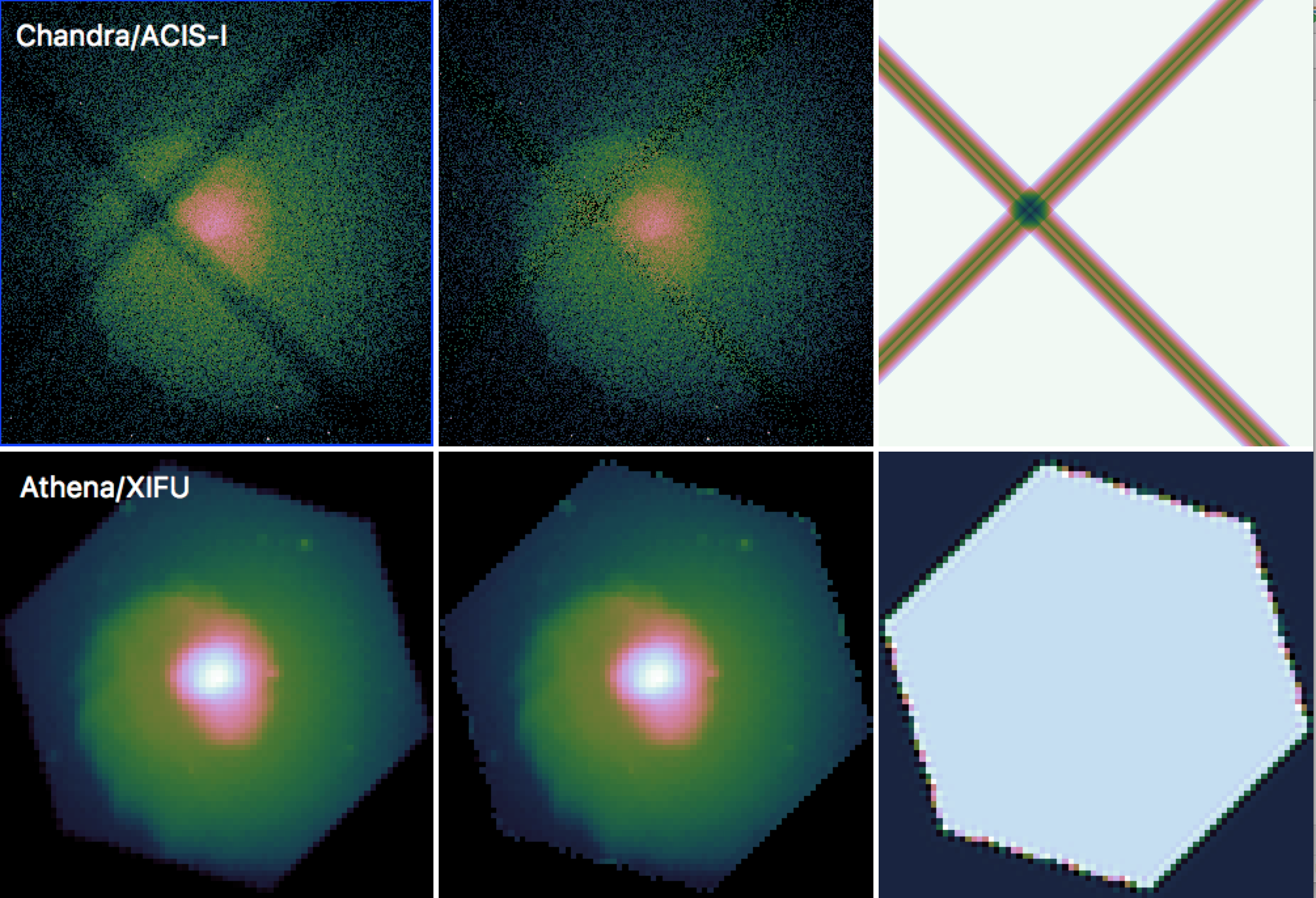
Figure 1: Images (left), exposure-corrected images (center) and exposure maps (right) for mock observations of a galaxy cluster for Chandra/ACIS-I (top) and Athena/XIFU (bottom), simulated using SOXS.
Warning
The make_exposure_map() tool only produces exposure maps for event
files produced by SOXS, and this is the only tool that should be used for this purpose
for event files produced by SOXS.
write_image
write_image() bins up events into an image according to the coordinate
system inherent in the event file and writes the image to a FITS file. Images of sky, detector,
or chip coordinates can be written. You can also restrict events within a particular energy range
or time range to be written to the file.
To write an image in sky coordinates:
from soxs import write_image
# Energy bounds are in keV
write_image("my_evt.fits", "my_sky_img.fits", emin=0.5, emax=7.0)
Or in detector coordinates:
write_image("my_evt.fits", "my_det_img.fits", coord_type='det', emin=0.5, emax=7.0)
To filter on a time range:
write_image("my_evt.fits", "my_sky_img.fits", emin=0.5, emax=7.0, tmin=0.0,
            tmax=(200.0, "ks"))
To filter on multiple energy bands, use a list of tuples of minimum, maximum energy of
each band (in keV) supplied to the bands keyword (this is an alternative to emin and
emax, and if present will override them:
write_image("my_evt.fits", "my_sky_img.fits", bands=[(0.5, 2.0), (4.0, 6.0)])
To supply an exposure map produced by make_exposure_map() to make a
flux image:
write_image("my_evt.fits", "my_sky_img.fits", coord_type='sky', emin=0.5, emax=7.0,
            expmap_file="my_expmap.fits")
To bin at a pixel size 4 times larger than the native pixel size, set reblock to 4:
write_image("my_evt.fits", "my_sky_img.fits", coord_type='sky', emin=0.5, emax=7.0,
            expmap_file="my_expmap.fits", reblock=4)
Note that if you set reblock and supply an exposure map, it must have been made with
the same value of reblock.
make_image
make_image() is almost identical to write_image(),
but it does not request an output filename. Instead, it bins up events into an image
according to the coordinate system inherent in the event file and returns an
ImageHDU object. Otherwise, the rest of the arguments to
make_image() are the same as to write_image().
write_radial_profile
write_radial_profile() bins up events into an radial profile defined by source
center, a minimum radius, a maximum radius, and a number of bins. One can restrict the events that
are binned by a specific energy band. An example execution:
from soxs import write_radial_profile
ctr = [30.0, 45.0] # by default the center is in celestial coordinates
rmin = 0.0 # arcseconds
rmax = 100.0 # arcseconds
nbins = 100 # number of bins
emin = 0.5 # keV
emax = 2.0 # keV
write_radial_profile("my_evt.fits", "my_radial_profile.fits", ctr, rmin,
                     rmax, nbins, emin=emin, emax=emax, overwrite=True)
If one wants to specify a center in physical pixel coordinates, you can use the same execution but
set the ctr_type keyword to “physical” and use physical pixel coordinates as the ctr argument:
from soxs import write_radial_profile
ctr = [2048.5, 2048.5] # by default the center is in celestial coordinates
rmin = 0.0 # arcseconds
rmax = 100.0 # arcseconds
nbins = 100 # number of bins
emin = 0.5 # keV
emax = 2.0 # keV
write_radial_profile("my_evt.fits", "my_radial_profile.fits", ctr, rmin,
                     rmax, nbins, ctr_type="physical", emin=emin, emax=emax,
                     overwrite=True)
If one wants to compute flux-based quantities for the radial profile (such as surface flux),
supply an exposure map produced by make_exposure_map():
write_radial_profile("my_evt.fits", "my_radial_profile.fits", ctr, rmin,
                     rmax, nbins, ctr_type="physical", emin=emin, emax=emax,
                     expmap_file="my_expmap.fits", overwrite=True)
A cookbook example showing how to extract a radial profile is shown in Radial Profile.
write_spectrum
write_spectrum() bins up events into a spectrum and writes the spectrum
to a FITS file:
from soxs import write_spectrum
write_spectrum("my_evt.fits", "my_spec.pha", overwrite=True)
This spectrum file can be read and fit with standard X-ray analysis software such as XSPEC, ISIS, and Sherpa.
To filter out events based on position for the spectrum, we can use a region file from ds9, CIAO, etc.:
write_spectrum("my_evt.fits", "my_spec.pha", region="circle.reg",
               overwrite=True)
Alternatively, you can use a region string:
reg = '# Region file format: DS9\nimage\ncircle(147.10,254.17,3.1) # color=green\n'
write_spectrum("my_evt.fits", "my_spec.pha", region=reg, overwrite=True)
Filtering on a time or energy range is also possible:
write_spectrum("my_evt.fits", "my_spec.pha", emin=0.5, emax=2.0,
               tmin=0.0, tmax=(0.5, "Ms"), overwrite=True)
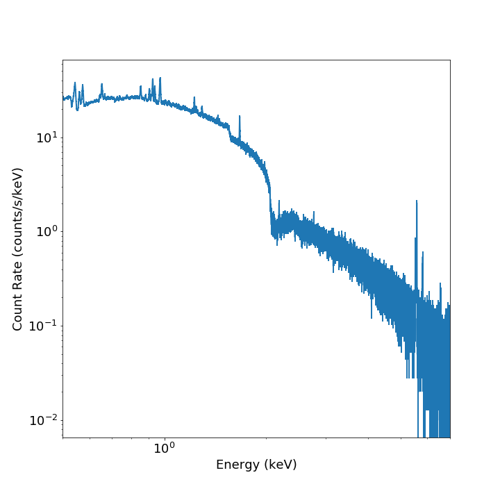
plot_spectrum
plot_spectrum() reads a spectrum stored in a FITS table file and makes
a Matplotlib plot. There are a number of options for
customizing the plot in the call to plot_spectrum(), but the method
also returns the Figure and the Axes
objects to allow for further customization. This example opens up a spectrum file and plots
it between 0.5 and 7.0 keV:
from soxs import plot_spectrum
fig, ax, ebins = plot_spectrum("evt.pha", xmin=0.5, xmax=7.0)
Note that in addition to the Figure and Axes
objects, the energy bin edges are also returned.
If one wanted to plot the same spectrum in channel space instead of energy space, you
would set plot_energy=False:
from soxs import plot_spectrum
fig, ax, ebins = plot_spectrum("evt.pha", plot_energy=False, xmin=300, xmax=7000)

where in that case the x-axis is now in channel space, so xmin and xmax had to
be set accordingly.
The spectrum will be plotted using points by default, but it is also possible to make
a step plot instead by setting plot_steps=True:
from soxs import plot_spectrum
fig, ax, ebins = plot_spectrum("evt.pha", plot_steps=True)
Rebinning on Energy
By default, the energy bins of the plot correspond to the bin edges of the channels.
It is also possible to customize the energy binning of the plot in three different
ways, via the ebins keyword argument. The first way is to simply provide a
NumPy array of energy bin edges that you constructed:
from soxs import plot_spectrum
import numpy as np
ebins = np.linspace(0.5, 7.0, 101)
fig, ax, ebins_out = plot_spectrum("evt.pha", ebins=ebins, xmin=0.5, xmax=7.0)
Another way to set the energy bins is to set ebins to an integer, which will
cause the spectrum to be reblocked by that factor:
from soxs import plot_spectrum
import numpy as np
ebins = 4 # energy bins contain 4 channels each
fig, ax, ebins_out = plot_spectrum("evt.pha", ebins=ebins, xmin=0.5, xmax=7.0)
The third way to set the energy bins is to provide a 2-tuple to ebins, where the
first element is the minimum significance (assuming Poisson statistics) of each bin
and the second element is the maximum number of channels to be combined in the bin:
from soxs import plot_spectrum
import numpy as np
ebins = (3.0, 4) # bins have 3-sigma significance and contain no more than 4 channels
fig, ax, ebins_out = plot_spectrum("evt.pha", ebins=ebins, xmin=0.5, xmax=7.0)
For other customizations, consult the plot_spectrum() API.
plot_image
The plot_image() function allows one to plot an image from a FITS
file. Several examples of this are shown in the following cookbook recipes:
For the full range of customizations, consult the plot_image() API.
merge_event_files
soxs.events.tools.merge_event_files() can be used to merge several event files
together. This may be useful if you want to merge a source file with a background
file created later, for example.
soxs.merge_event_files(["src1_evt.fits", "src2_evt.fits", "bkg_evt.fits"],
                       "merged_evt.fits", overwrite=True)
fill_regions
fill_regions() can be used to fill in regions with background
counts in an image which has had bright sources removed by a tool such as
wavdetect. In addition to
the file containing the image to be filled and the name of the new file to be written,
the user supplies a region or list of regions to fill in (region strings, ds9 region
files, Region objects, or a Regions object), and
bkg_value, which is either a single floating-point value for the number of
background counts, a single region from which to get this number, or a list of regions
(of the same number as the source list of regions) to obtain this number from. By
default, bkg_value number for each region will serve as the mean of a Poisson
distribution from which random numbers of counts will be drawn for each pixel in
each region to be filled. If a region or regions are supplied for bkg_value,
by default the mean number of counts from each region will be used to calculate this
value, though it is also possible to use the median value.
Here is an example where we want to fill a single region with the counts where the mean from is taken another region:
soxs.fill_regions("holed_img.fits", "filled_img.fits", "src.reg", "bkg.reg",
                  overwrite=True)
Here is the same example, except that we use the median number of counts within
"bkg.reg" to determine the mean of the Poisson distribution to fill with:
soxs.fill_regions("holed_img.fits", "filled_img.fits", "src.reg", "bkg.reg",
                  median=True, overwrite=True)
Here is an example where we fill the hole supplying a single number for the mean of the Poisson distribution:
soxs.fill_regions("holed_img.fits", "filled_img.fits", "src.reg", 10.0,
                  overwrite=True)