Cosmological Source Catalog

SOXS provides the make_cosmological_sources_file() function to generate a set of photons from cosmological halos and store them in a SIMPUT catalog.

First, import our modules:

import matplotlib

matplotlib.rc("font", size=18)
import soxs

Second, define our parameters, including the location within the catalog where we are pointed via the argument cat_center. To aid in picking a location, see the halo map.

exp_time = (200.0, "ks")
fov = 20.0  # in arcmin
sky_center = [30.0, 45.0]  # in degrees
cat_center = [3.1, -1.9]

Now, use make_cosmological_sources_file() to create a SIMPUT catalog made up of photons from the halos. We’ll set a random seed using the prng parameter to make sure we get the same result every time. We will also write the halo properties to an ASCII table for later analysis, using the output_sources parameter:

soxs.make_cosmological_sources_file(
    "my_cat.simput",
    "cosmo",
    exp_time,
    fov,
    sky_center,
    cat_center=cat_center,
    prng=33,
    overwrite=True,
)

soxs : [INFO     ] 2026-01-06 13:38:08,480 Creating photons from cosmological sources.
soxs : [INFO     ] 2026-01-06 13:38:08,481 Loading halo data from catalog: /Users/jzuhone/Source/soxs/soxs/files/halo_catalog.h5
soxs : [INFO     ] 2026-01-06 13:38:08,540 Coordinates of the FOV within the catalog are (3.1, -1.9) deg.
soxs : [INFO     ] 2026-01-06 13:38:08,541 Selecting halos in the FOV.
soxs : [INFO     ] 2026-01-06 13:38:08,544 Number of halos in the field of view: 384

soxs : [INFO     ] 2026-01-06 13:38:15,917 Created 5786907 photons from cosmological sources.
soxs : [INFO     ] 2026-01-06 13:38:15,981 Appending source 'cosmo' to my_cat.simput.

<soxs.simput.SimputCatalog at 0x1135a7e00>

Next, use the instrument_simulator() to simulate the observation:

soxs.instrument_simulator(
    "my_cat.simput",
    "cosmo_cat_evt.fits",
    exp_time,
    "lynx_hdxi",
    sky_center,
    overwrite=True,
)

soxs : [INFO     ] 2026-01-06 13:38:16,127 Simulating events from 1 sources using instrument lynx_hdxi for 200 ks.
soxs : [INFO     ] 2026-01-06 13:38:16,948 Scattering energies with RMF xrs_hdxi.rmf.

soxs : [INFO     ] 2026-01-06 13:38:19,096 Detected 2164879 events in total.
soxs : [INFO     ] 2026-01-06 13:38:19,104 Adding background events.
soxs : [INFO     ] 2026-01-06 13:38:19,157 Adding in point-source background.
soxs : [INFO     ] 2026-01-06 13:38:30,544 Simulating events from 1 sources using instrument lynx_hdxi for 200 ks.
soxs : [INFO     ] 2026-01-06 13:38:34,448 Scattering energies with RMF xrs_hdxi.rmf.

soxs : [INFO     ] 2026-01-06 13:38:38,500 Detected 4694277 events in total.
soxs : [INFO     ] 2026-01-06 13:38:38,516 Generated 4694277 photons from the point-source background.
soxs : [INFO     ] 2026-01-06 13:38:38,516 Adding in astrophysical foreground.

soxs : [INFO     ] 2026-01-06 13:38:47,342 Adding in instrumental background.
soxs : [INFO     ] 2026-01-06 13:38:48,898 Making 34150396 events from the galactic foreground.
soxs : [INFO     ] 2026-01-06 13:38:48,899 Making 522961 events from the instrumental background.
soxs : [INFO     ] 2026-01-06 13:38:54,826 Observation complete.
soxs : [INFO     ] 2026-01-06 13:38:54,827 Writing events to file cosmo_cat_evt.fits.

We can use the write_image() function in SOXS to bin the events into an image and write them to a file, restricting the energies between 0.7 and 7.0 keV:

soxs.write_image(
    "cosmo_cat_evt.fits", "cosmo_img.fits", emin=0.7, emax=7.0, overwrite=True
)

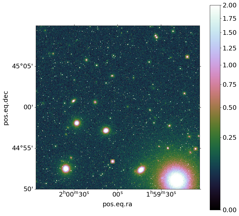
We can now show the resulting image:

fig, ax = soxs.plot_image(
    "cosmo_img.fits",
    stretch="sqrt",
    cmap="cubehelix",
    vmin=0.0,
    vmax=2.0,
    width=0.33333,
)