Simulating Source Catalogs
SOXS has the capability of simulating two different types of source catalogs: X-rays from a population of halos (galaxies, galaxy groups, and galaxy clusters), and point sources.
Cosmological Source Catalog
SOXS provides a routine to generate X-ray photons from cosmologically distant sources. This is made possible using a halo catalog provided by Daisuke Nagai (Yale) and Masato Shirasaki (NAOJ). The halo catalog is extracted from a light cone simulation produced using the methods of Shirasaki et al. (2015). It includes \(M_{500c}\), \(z\), and center coordinates for each halo.
The light cone simulation of \(10 \times 10\) square degrees is produced from two N-body simulation boxes with \(L = 480~\rm{Mpc/h}\) and \(L = 960~\rm{Mpc/h}\), out to the maximum redshift of z = 3, performed with the Gadget-2 code (Springel 2005). Each simulation box contains \(1024^3\) dark matter particles. Halo finding was performed using Rockstar (Behroozi et al. 2013), and only host halos were used and not subhalos.
The cosmological parameters for this halo catalog are from the WMAP 9-year cosmology Hinshaw et al. 2013:
\(h = 0.7\)
\(\Omega_m = 0.279\)
\(\Omega_\Lambda = 0.721\)
\(\Omega_b = 0.0463\)
\(w_{\rm DE} = -1\)
\(\sigma_8 = 0.823\)
\(n_s = 0.972\)
The X-ray emitting intracluster medium for each halo is modeled using a \(\beta\)-model function for the surface brightness and assuming isothermality. Using scaling relations from Vikhlinin et al. (2009), the halo temperature and flux are derived from the halo mass and redshift, assuming an APEC model for the spectrum. The scale radius of each halo is given by \(r_{500c}/10\). The \(\beta\)-parameter for each halo is drawn from a normal distribution with mean 2/3 and standard deviation 0.05. Each halo is also given a random ellipticity from a Gaussian distribution of mean 0.85 and standard deviation 0.15, and the orientation of this ellipticity is drawn from a uniform distribution over the range \([0, 2\pi]\).
A low-mass cut has been made at \(M_{500c} = 3 \times 10^{12}~M_\odot\).
Flat-Field Map of Structure
Below is a map showing an image of the full flat-field \(10 \times 10\) degree sky flux map (in the 0.5-2 keV band) of the X-ray halos in the catalog.
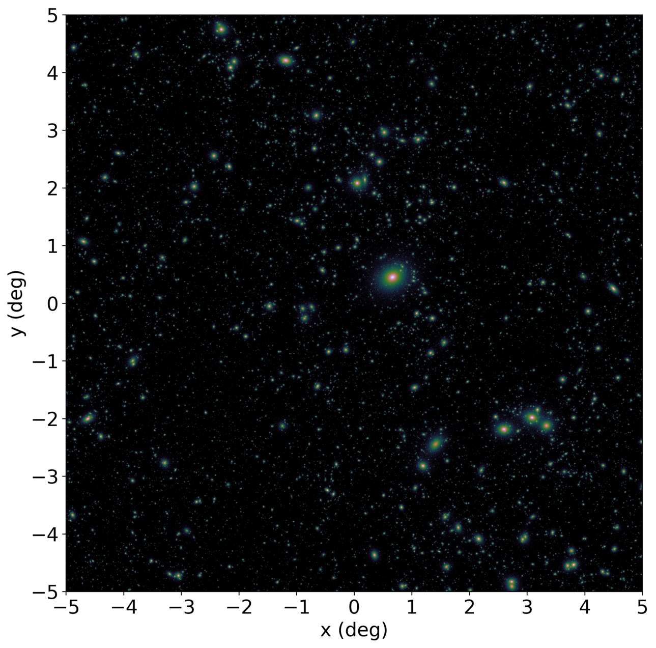
A FITS image of this map (in units of \(\rm{photons~s^{-1}~cm^{-2}}\) in the
0.5-2 keV band) can be downloaded from the link below, which you can open in ds9
to select regions of interest and determine coordinates to be passed into the
cat_center parameter of make_cosmological_sources_file().
A full ASCII table of the halos in the catalog and their properties is also provided.
Note
In the observations you create, the ellipticities and orientations of the halos will be different from those in this map. This map is provided as a convenience to locate which regions may show interesting structure.
make_cosmological_sources_file
make_cosmological_sources_file() generates a photon list
file for a SIMPUT catalog using the cosmological sources model:
filename = "cosmo.simput"
name = "my_cosmo_sources"
exp_time = (500.0, "ks")
fov = 20.0 # arcmin
sky_center = [30.0, 45.0] # RA, Dec in degrees
absorb_model = "wabs" # Choose a model for absorption, optional
nH = 0.02 # Foreground galactic absorption, optional
area = (4.0, "m**2") # Flat collecting area to generate photon sample
soxs.make_cosmological_sources_file(filename, name, exp_time, fov, sky_center,
                                    absorb_model=absorb_model, nH=nH,
                                    area=area)
To append to an existing catalog filename, set append=True. If you
want to write the cosmological sources to a separate file, use the
src_filename keyword argument.
By default, a random position will be chosen within the halo catalog. If you
would prefer to simulate a specific region within the catalog, set the keyword
argument cat_center to a particular coordinate between [-5, 5] degrees in
either direction:
cat_center = [-0.2, 3.0]
soxs.make_cosmological_sources_file(filename, name, exp_time, fov, sky_center,
                                    absorb_model=absorb_model, nH=nH,
                                    area=area, cat_center=cat_center)
One can also write out ds9 circle regions corresponding to
the positions of the halos on the sky, with the radii of the circles given by the
\(r_{500}\) of the halos, using the write_regions argument:
soxs.make_cosmological_sources_file(filename, name, exp_time, fov, sky_center,
                                    absorb_model=absorb_model, nH=nH,
                                    area=area, write_regions="halos.reg")
Point Source Catalog
SOXS also provides a function to create a SIMPUT catalog of point-sources. It is not necessary to do this for including point sources as a background component in SOXS, as this will be done automatically, but it may be useful if you would like to tweak parameters of the sources, store the positions and fluxes of the sources generated, or use the SIMPUT catalog in another simulation program such as MARX or SIMX.
make_point_sources_file() generates a
photon list file for a SIMPUT catalog using the point-source background model
described in Point Source Background Model:
filename = "pt_src.simput"
name = "my_point_sources"
exp_time = (500.0, "ks")
fov = 20.0 # arcmin
sky_center = [30.0, 45.0] # RA, Dec in degrees
absorb_model = "tbabs" # Choose a model for absorption, optional
nH = 0.02 # Foreground galactic absorption, optional
area = (4.0, "m**2") # Flat collecting area to generate photon sample
soxs.make_point_sources_file(filename, name, exp_time, fov, sky_center,
                             absorb_model=absorb_model, nH=nH,
                             area=area)
To append to an existing catalog filename, set append=True. If you
want to write the cosmological sources to a separate file, use the
src_filename keyword argument.
A uniform background across the field of view, associated with many completely
unresolved point sources, is also added, with a spectral index of \(\alpha = 2.0\)
and a flux of \(1.352 \times 10^{-12}~\rm{erg}~\rm{s}^{-1}~\rm{cm}^{-2}~\rm{deg}^{-2}\)
in the 0.5-2 keV band. This can be turned off by setting diffuse_unresolved=False in the
call to make_point_sources_file().
Saving the Point Source Properties to Disk for Later Use
One can also save the point-source properties to disk for examination or later use
to generate a consistent set of point sources more than once. This can be done in two
different ways. The first is via make_point_sources_file()
itself, using the output_sources keyword argument:
filename = "pt_src.simput"
name = "my_point_sources"
exp_time = (500.0, "ks")
fov = 20.0 # arcmin
sky_center = [30.0, 45.0] # RA, Dec in degrees

soxs.make_point_sources_file(filename, name, exp_time, fov,
                             sky_center, output_sources="my_srcs.dat")
This saves the point source properties of position, flux, and spectral index
to an ASCII table file, as a side effect of generating the point source events.
However, one may want to simply generate this table without generating events,
so SOXS also provides the make_point_source_list()
method:
output_file = "my_srcs.dat"
fov = 20.0 # arcmin
sky_center = [30.0, 45.0] # RA, Dec in degrees

soxs.make_point_source_list(output_file, fov, sky_center)
Regardless of which method used, this ASCII table can be used as input to
make_point_sources_file() via the
input_sources keyword argument, e.g.:
filename = "pt_src.simput"
name = "my_point_sources"
exp_time = (500.0, "ks")
fov = 20.0 # arcmin
sky_center = [30.0, 45.0] # RA, Dec in degrees

soxs.make_point_sources_file(filename, name, exp_time, fov,
                             sky_center, input_sources="my_srcs.dat")
Which ensures that one would have the same set of point sources every time it is
run. You can also pass this file to the input_pt_sources keyword argument of
instrument_simulator() or
make_background_file().
Both of the functions make_point_sources_file()
and make_point_source_list() also take the
drop_brightest option, which if set to an integer will drop the specified
number of brightest sources from the list (this is a poor-person’s version of
removing point sources from observations):
filename = "pt_src.simput"
name = "my_point_sources"
exp_time = (500.0, "ks")
fov = 20.0 # arcmin
sky_center = [30.0, 45.0] # RA, Dec in degrees

# drop the 50 brightest sources
soxs.make_point_sources_file(filename, name, exp_time, fov,
                             sky_center, drop_brightest=50)