Instrument Simulation in SOXS
Running the Instrument Simulator
The end product of a mock observation is a “standard” event file which has been convolved with a model for the telescope. In SOXS, this is handled by the instrument simulator.
instrument_simulator() reads in a SIMPUT catalog or
pyXSIM event list and creates a standard event file using the instrument simulator.
instrument_simulator() performs the following actions:
Uses the effective area curve to determine which events will actually be detected.
Projects these events onto the detector plane and perform PSF blurring and dithering of their positions (if dithering is enabled for that particular instrument).
Add background events.
Convolves the event energies with the response matrix to produce channels.
Writes everything to an event file.
If the input events are a SIMPUT catalog, then all of the SIMPUT sources,
whether spectra or photon lists, will be processed. Alternatively, a pyXSIM
event list in the HDF5 format can be supplied as a source. A typical
invocation of instrument_simulator() using a SIMPUT
catalog looks like the following:
import soxs
source_file = "snr_simput.fits" # SIMPUT file to be read
out_file = "evt_lxm.fits" # event file to be written
exp_time = (30.0, "ks") # The exposure time
instrument = "lynx_lxm" # short name for instrument to be used
sky_center = [30., 45.] # RA, Dec of pointing in degrees
soxs.instrument_simulator(source_file, out_file, exp_time, instrument,
                          sky_center, overwrite=True)
and in the case of a pyXSIM event file:
import soxs
source_file = "sloshing_photons.h5" # pyXSIM events file to be read
out_file = "evt_acis.fits" # event file to be written
exp_time = (100.0, "ks") # The exposure time
instrument = "chandra_acisi_cy0" # short name for instrument to be used
sky_center = [30., 45.] # RA, Dec of pointing in degrees
soxs.instrument_simulator(source_file, out_file, exp_time, instrument,
                          sky_center, overwrite=True)
The overwrite argument allows an existing file to be overwritten. We now
describe instrument simulation in more detail.
The instrument Argument
SOXS currently supports a number of instrument configurations “out of the box”.
Any of these can be specified with the instrument argument:
Lynx
All Lynx configurations correspond to the \(d = 3~m, f = 10~m\) mirror system.
Imaging
For Lynx, there are currently four base imaging instruments, "lynx_hdxi"
for the High-Definition X-ray Imager (HDXI), and the three subarrays of the
Lynx X-ray Microcalorimeter (LXM): the Main Array ("lynx_lxm"), the
Enhanced Main Array ("lynx_lxm_enh"), and the Ultra High-Resolution Array
("lynx_lxm_ultra").
The HDXI has a single square-shaped 20-arcminute field of view, and the three different subarrays for the LXM have different plate scales, field of view, and spectral resolutions. They are:
"lynx_lxm": 5’ field of view, 1” pixels, 3 eV spectral resolution"lynx_lxm_enh": 1’ field of view, 0.5” pixels, 1.5 eV spectral resolution"lynx_lxm_ultra": 1’ field of view, 1” pixels, 0.3 eV spectral resolution (restricted to energies below ~1 keV)
The default instrumental background in SOXS for the "lynx_hdxi" model is the
Chandra/ACIS-I particle background, and the default instrumental background
for the "lynx_lxm_*" models is based on a model developed for the Athena
calorimeter
(see here for details).
Gratings
A single gratings instrument specification for Lynx is included with SOXS,
the Lynx X-ray Gratings Spectrometer, "lynx_xgs", which currently only
allows simulations of spectra. It corresponds approximately to the
\(d = 3~m, f = 10~m\) mirror system, 50% coverage of the input aperture
by the gratings, and \(R = 5000\).
Athena
For simulating Athena observations, two instrument specifications are available, for the WFI (Wide-Field Imager) and the X-IFU (X-ray Integral Field Unit). For both of these specifications, a 12-meter focal length is assumed. The PSF model, response files, and background models are used from the SIXTE software package. The WFI detector consists of four chips laid out in a 2x2 shape with a field of view of approximately 40 arcminutes, and the X-IFU detector has a single hexagonal shape with an approximate diameter of 5 arcminutes.
Chandra
For simulating Chandra observations, a number of instrument specifications are available. All specifications assume a 10-meter focal length, dithering, and 0.492-arcsecond pixels. They also include a simplified model for the on and off-axis Chandra PSF.
The default instrumental background in SOXS for the Chandra ACIS-I models is the Chandra/ACIS-I particle background. For ACIS-S, the ACIS-I background is used for the front-illuminated chips, and a model provided by Andrea Botteon from Botteon et al. 2017 is used for the back-illuminated chips. Currently, the gratings instrument models do not have instrumental backgrounds included.
ACIS-I
The four ACIS-I specifications have a square field of view laid out in four
chips 8 arcminutes on a side arranged 2x2. The four different separate
specifications correspond to different observing cycles: 0, 10, 22, and 28.
Each specification is named with a keyword of the form "chandra_acisi_cyN",
where N is the cycle number. For example, "chandra_acisi_cy22" corresponds
to the instrument configuration from Cycle 22. The main effect of the different
cycles is that the effective area at low energies for "chandra_acisi_cy22"
is much lower at later times due to the buildup of contamination on the ACIS
optical blocking filters.
ACIS-S
The two ACIS-S specifications have 6 chips 8 arcminutes on a side in a single
row. As in the ACIS-I case, the specifications are for Cycles 0, 10, 22, and 28,
and are named with the same convention, e.g. "chandra_aciss_cy22" for the
Cycle 22 configuration.
HETG
Eight gratings specifications have been included for ACIS-S and the HETG, for both Cycle 0 and Cycle 22. These simulate spectra only for the MEG and HEG, for the \(\pm\) first order spectra. They are named:
"chandra_aciss_meg_m1_cy0""chandra_aciss_meg_p1_cy0""chandra_aciss_heg_m1_cy0""chandra_aciss_heg_p1_cy0""chandra_aciss_meg_m1_cy22""chandra_aciss_meg_p1_cy22""chandra_aciss_heg_m1_cy22""chandra_aciss_heg_p1_cy22"
XRISM
A number of instrument specifications are available for XRISM.
All but one of these are for the Resolve instrument. Each Resolve specification has a ~3 arcminute square FoV with 6 pixels on a side. The differences between the specifications depend on the resolution of the RMF and the presence or absence of a filter. The three instrument specifications which vary by RMF resolution are:
"xrism_resolve_Hp_5eV": High-resolution RMF with 5 eV resolution"xrism_resolve_Mp_7eV": Medium-resolution RMF with 6 eV resolution"xrism_resolve_Lp_18eV": Low-resolution RMF with 18 eV resolution
All of these have no filter. For each of these RMF resolution options, there is
are versions for the Beryllium filter, e.g. "xrism_resolve_fwBe_Hp_5eV", and for
the neutral density filter, e.g. "xrism_resolve_fwND_Lp_18eV". All Resolve
instrument specifications assume the gate valve is closed. These specifications use a
image-based PSF model with a FWHM of ~1.2” arcminutes.
The "xrism_resolve" specification is mapped directly to the "xrism_resolve_Hp_5eV"
specification. An otherwise identical specification, "xrism_resolve_1arcsec", has
a Gaussian PSF with 1 arcsecond FWHM.
For the Xtend instrument, the "xrism_xtend" specification has 2x2 CCDs laid
out in a ~38’ FoV, with a pixel size of ~1.77”.
The response files, PSF models, and instrumental background models used for XRISM in SOXS were obtained from here.
AXIS
A single instrument specification "axis" is available for
AXIS, the Advanced X-ray Imaging Satellite.
The specification is for the wide-field imaging instrument, with a 27.1’ field of
view, 2x2 CCD array configuration, and a 9 m focal length. Response files, the
PSF model, and the instrumental background model have been provided by Eric
Miller of MIT.
STAR-X
A single instrument specification "star-x" is available for
*STAR-X*.
The specification is for the wide-field imaging istrument, with a 1 degree field
of view, a 4.5 m focal length, and a Gaussian PSF with a FWHM of 3 arcseconds.
Currently, no instrumental background is included. The response files for
STAR-X were provided by Michael McDonald.
Line Emission Mapper (LEM)
Two instrument specifications "lem_outer_array" and "lem_inner_array", are
available for the Line Emission Mapper (LEM)
mission concept. Both have a 4 m focal length and a Gaussian PSF with a FWHM
of 10 arcseconds. The outer array has a square-shaped 32 arcminute field of view
and a spectral resolution of 2.5 eV, whereas the inner array has a square-shaped
7 arcminute field of view and a spectral resolution of 1.3 eV. The old LEM
configurations "lem_2eV" and "lem_0.9eV" are still supported, both with
square fields of view of 32 arcminutes.
Explorer of Cosmic Ecosystems and Energetic Dynamics (ExCEED)
Two instrument specifications "exceed_outer_array" and "exceed_inner_array",
are available for the Explorer of Cosmic Ecosystems and Energetic Dynamics
(ExCEED) mission concept. Both have a 4 m focal length and a Gaussian PSF with
a FWHM of 10 arcseconds. The outer array has a square-shaped 32 arcminute field
of view and a spectral resolution of 2.5 eV, whereas the inner array has a
square-shaped 7-arcminute field of view and a spectral resolution of 1.3 eV. The
effective area curve for ExCEED is derived from a mirror model produced by COSINE,
detailed in
Barrière et al. (2025).
Backgrounds
The instrument simulator simulates background events as well as the source
events provided by the user. There are three background components: the
Galactic foreground, a background comprised of discrete point sources, and the
instrumental/particle background. Complete information about these components
can be found in Background Models in SOXS, but here the keyword arguments pertaining to
backgrounds for instrument_simulator() will be detailed.
The various background components can be turned on and off using
the ptsrc_bkgnd, instr_bkgnd, and foreground arguments. They are all
on by default, but can be turned on or off individually:
# turns off the astrophysical background but leaves in the instrumental
instrument_simulator(simput_file, out_file, exp_time, instrument,
                     sky_center, overwrite=True, instr_bkgnd=False,
                     foreground=True) # ptsrc_bkgnd True by default
For long exposures, backgrounds may take a long time to generate. For this
reason, SOXS provides a way to add a background stored in a previously
generated event file to the simulation of a source, via the bkgnd_file
argument:
# loads the background from a file
instrument_simulator(simput_file, out_file, exp_time, instrument,
                     sky_center, overwrite=True, bkgnd_file="my_bkgnd.fits")
In this case the values of instr_bkgnd, ptsrc_bkgnd, and foreground
are ignored regardless of their value. The required background event file can be
generated using make_background_file(), and is documented
at Using a Background From an Event File. The background event file must be for the same instrument
as the one that is being simulated for the source and must have an exposure time
at least as long as the source exposure.
Coordinate Systems in SOXS
SOXS event files produced by the instrument simulator have two coordinate
systems: the (X, Y) “sky” coordinate system and the (DETX, DETY) “detector”
coordinate system. The original RA and Dec of the simulated photons, before
any scattering of the photon positions by the PSF or dithering, are stored
in the event file as columns "RA_ORIG" and "DEC_ORIG" for reference.
For a given instrument, the detector coordinate system is defined by a square field of view divided into a number of pixels on each side. The field of view is shown in the schematic diagram in Figure 1 as the dashed red square. The center of the field of view has detector coordinates 0,0, as can be seen in Figure 1.
The sky coordinate system is defined to be twice the size of the field of view,
with twice as many pixels. The center of the sky coordinate system is given by
pixel coordinates 0.5*(2*num_pixels+1),0.5*(2*num_pixels+1). The sky
coordinate system is also shown in Figure 1. In event files and images, standard
world coordinate system (WCS) keywords are used to translate between sky
coordinates and RA and Dec.
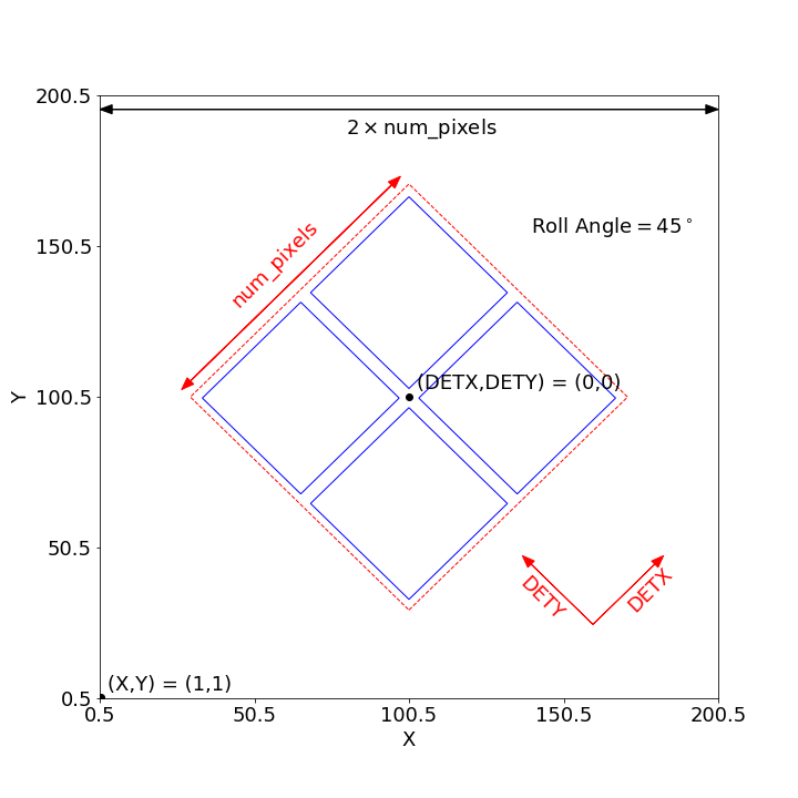
Figure 1: Schematic showing the layout of sky and detector coordinate systems, as well as multiple chips, for an example instrument similar to Chandra/ACIS-I. A roll angle of 45 degrees has been specified.
If the roll_angle parameter of the instrument simulation is 0, the sky and
detector coordinate systems will be aligned, but otherwise they will not. Figure
1 shows the orientation of the detector in the sky coordinate system for a roll
angle of 45 degrees. For observations which have dither, the sky coordinates and
the detector coordinates will not have a one-to-one mapping, but will change as
a function of time.
Finally, Figure 1 also shows that multiple “chips” can be specified. In SOXS, chips are simply elements which are capable of detecting X-ray photons. Only events which fall within chip regions are detected. For more information on how multiple chips can be specified for a particlular instrument, see Defining Chips.
Warning
At the present time, the coordinate systems specified in SOXS do not correspond directly to those systems in event files produced by actual X-ray observatories. This is particularly true of detector coordinates. The conventions chosen by SOXS are mainly for convenience.
Other Modifications
You can also change other aspects of the observation with
instrument_simulator(). For example, you can change the
size and period of the Lissajous dither pattern, for instruments which have
dithering enabled. The default dither pattern has amplitudes of 8.0 arcseconds
in the DETX and DETY directions, and a period of 1000.0 seconds in the DETX
direction and a period of 707.0 seconds in the DETY direction. You can change
these numbers by supplying a list of parameters to the dither_params
argument:
import soxs
# The order of dither_params is [x_amp, y_amp, x_period, y_period]
# the units of the amplitudes are in arcseconds and the periods are in
# seconds
dither_params = [8.0, 16.0, 1000.0, 2121.0]
soxs.instrument_simulator(simput_file, out_file, exp_time, instrument,
                          sky_center, overwrite=True,
                          dither_params=dither_params)
To turn dithering off entirely for instruments that enable it, use the
no_dither argument:
import soxs
soxs.instrument_simulator(simput_file, out_file, exp_time, instrument,
                          sky_center, overwrite=True,
                          no_dither=True)
Note
Dithering will only be enabled if the instrument specification allows for it. For example, for Lynx, dithering is on by default, but for XRISM it is off.
To move the aimpoint of the observation away from the nominal aimpoint on the
detector, use the aimpt_shift argument, which is a two-element array of
numbers (assumed units of arcseconds) which will shift the aimpoint by those
values:
import soxs
soxs.instrument_simulator(simput_file, out_file, exp_time, instrument,
                          sky_center, overwrite=True,
                          aimpt_shift=[10.0,-20.0])
Simulating Spectra Only
If you would like to use an instrument specification and a
Spectrum object to generate a spectrum file only (without
including spatial effects), SOXS provides a function
simulate_spectrum() which can take an unconvolved
spectrum and generate a convolved one from it. This is similar to what the XSPEC
command “fakeit” does.
spec = soxs.Spectrum.from_file("lots_of_lines.dat")
instrument = "lynx_lxm"
out_file = "lots_of_lines.pha"
simulate_spectrum(spec, instrument, exp_time, out_file, overwrite=True)
This spectrum file then can be read in and analyzed by standard software such as XSPEC, Sherpa, ISIS, etc.
The different background components that can be included in the
instrument_simulator() can also be used with
simulate_spectrum(). Because in this case the components
are assumed to be diffuse, it is necessary to specify an area on the sky
that the background was “extracted” from using the bkgnd_area parameter.
Here is an example invocation:
spec = soxs.Spectrum.from_file("lots_of_lines.dat")
instrument = "lynx_lxm"
out_file = "lots_of_lines.pha"
simulate_spectrum(spec, instrument, exp_time, out_file,
                  ptsrc_bkgnd=True, foreground=True,
                  instr_bkgnd=True, overwrite=True,
                  bkgnd_area=(1.0, "arcmin**2"))
However, there are a couple of differences. The first difference is that
backgrounds are turned off in simulate_spectrum() by
default, unlike in instrument_simulator(). The second
difference is that while for the instrument_simulator()
the point-source background is resolved into invdividual point sources, it is
not resolved for simulate_spectrum(), and instead is
modeled using an absorbed power-law with the following parameters:
Power-law index \(\alpha = 1.52\)
Normalization at 1 keV of \(f_{\rm CXB} 10^{-6}~\rm{photons~cm^{-2}~keV^{-1}}\), where \(f_{\rm CXB}\) is the fraction of the CXB that has been assumed to have been resolved into point sources and removed from the analysis. The default value for \(f_{\rm CXB} = 0.8\), but this can be changed by providing a different value to the
resolved_cxb_fracparameter in the call tosimulate_spectrum().Neutral hydrogen column of \(0.018 \times 10^{22}~\rm{cm}^{-2}\)
Here the tbabs model is assumed for the absorption. To change the default
absorption model or the neutral hydrogen column, use the SOXS Configuration File. Similarly,
the SOXS Configuration File can be used to change the APEC model version for the foreground.
Instrument specifications with the "imaging" keyword set to False can
only be used with simulate_spectrum(), and not
instrument_simulator(). Currently, this includes grating
instruments.
It is also possible to specify the instrument to use in the simulation with a 2 or 3-tuple giving the ARF, RMF, and (optionally) the background specification to use. This can be handy if you do not have anything but these files available, or if you are prototyping a new instrument specification. An example using the Lynx HDXI ARF and RMF:
instrument = ("xrs_hdxi_3x10.arf", "xrs_hdxi.rmf")
"bkgnd": ["lynx_hdxi_particle_bkgnd.pha", 1.0],
out_file = "hdxi_spec.pha"
simulate_spectrum(spec, instrument, exp_time, out_file,
                  ptsrc_bkgnd=True, foreground=True,
                  instr_bkgnd=False, overwrite=True,
                  bkgnd_area=(1.0, "arcmin**2"))
Note that this invocation has instr_bkgnd=False. If you want to include
a instrumental/particle background, you also need to specify the background
specifcation in the instrument tuple, which is a list including the name
of the background file and the normalization of the background in square
arcminutes:
instrument = (
    "xrs_hdxi_3x10.arf",
    "xrs_hdxi.rmf",
    ["lynx_hdxi_particle_bkgnd.pha", 1.0]
)
out_file = "hdxi_spec.pha"
simulate_spectrum(spec, instrument, exp_time, out_file,
                  ptsrc_bkgnd=True, foreground=True,
                  instr_bkgnd=True, overwrite=True,
                  bkgnd_area=(1.0, "arcmin**2"))
This way of using simulate_spectrum() is also useful
for creating models of particle backgrounds, if you have a background model and
would like to convolve it with an RMF. In this case, you can set the first
tuple element (the ARF) to None:
instrument = (
    None,
    "xrs_hdxi.rmf",
)
out_file = "hdxi_part_bkg.pha"
simulate_spectrum(spec, instrument, exp_time, out_file,
                  overwrite=True)
You can also adjust the overall normalization of the instrument background by
adjusting the keyword argument instr_bkgnd_scale, which has a default value of 1:
simulate_spectrum(spec, instrument, exp_time, out_file,
                  ptsrc_bkgnd=True, foreground=True,
                  instr_bkgnd=True, overwrite=True,
                  bkgnd_area=(1.0, "arcmin**2"),
                  instr_bkgnd_scale=0.5)
Finally, if you want to create a spectrum without counting (Poisson) statistics,
set noisy=False in the call to simulate_spectrum().
A Note About Simulations with Grating Instruments
Currently in SOXS, simulations of sources observed by grating instruments are
not supported with the instrument_simulator(). Gratings
observations can be generated using Spectrum objects
and simulate_spectrum(), which produces a mock gratings
spectrum:
import soxs

# Create an absorbed power-law spectrum
spec = soxs.Spectrum.from_powerlaw(2.0, 0.0, 0.1, 0.1, 10.0, 100000)
spec.apply_foreground_absorption(0.1, absorb_model='tbabs')

# Simulate the observed spectrum with Chandra/ACIS HETG: MEG, -1 order, Cycle 20
soxs.simulate_spectrum(spec, "chandra_aciss_meg_m1_cy20", (100.0, "ks"),
                       "soxs_meg_m1.pha", overwrite=True)

# Plot the spectrum
soxs.plot_spectrum("soxs_meg_m1.pha")
Adding particle backgrounds to grating instrument specifications in
simulate_spectrum() is not supported at this time.
Creating New Instrument Specifications
SOXS provides the ability to customize the models of the different components of the instrument being simulated. This is provided by the use of the instrument registry and JSON files which contain prescriptions for different instrument configurations.
The Instrument Registry
The instrument registry is simply a Python dictionary containing various
instrument specifications. You can see the contents of the instrument registry
by calling show_instrument_registry():
import soxs
soxs.show_instrument_registry()
gives (showing only a subset for brevity):
Instrument: lynx_hdxi
    name: lynx_hdxi
    arf: xrs_hdxi_3x10.arf
    rmf: xrs_hdxi.rmf
    bkgnd: ['lynx_hdxi_particle_bkgnd.pha', 1.0]
    fov: 22.0
    num_pixels: 4096
    aimpt_coords: [0.0, 0.0]
    chips: [['Box', 0, 0, 4096, 4096]]
    focal_length: 10.0
    dither: True
    psf: ['image', 'chandra_psf.fits', 6]
    imaging: True
    grating: False
Instrument: lynx_lxm
    name: lynx_lxm
    arf: xrs_mucal_3x10_3.0eV.arf
    rmf: xrs_mucal_3.0eV.rmf
    bkgnd: ['lynx_lxm_particle_bkgnd.pha', 1.0]
    fov: 5.0
    num_pixels: 300
    aimpt_coords: [0.0, 0.0]
    chips: [['Box', 0, 0, 300, 300]]
    focal_length: 10.0
    dither: True
    psf: ['image', 'chandra_psf.fits', 6]
    imaging: True
    grating: False
...
Instrument: athena_wfi
    name: athena_wfi
    arf: athena_sixte_wfi_wo_filter_v20190122.arf
    rmf: athena_wfi_sixte_v20150504.rmf
    bkgnd: ['sixte_wfi_particle_bkg_20190829.pha', 79552.92570677]
    fov: 40.147153
    num_pixels: 1078
    aimpt_coords: [53.69, -53.69]
    chips: [['Box', -283, -283, 512, 512],
            ['Box', 283, -283, 512, 512],
            ['Box', -283, 283, 512, 512],
            ['Box', 283, 283, 512, 512]]
    focal_length: 12.0
    dither: True
    psf: ['multi_image', 'athena_psf_15row.fits']
    imaging: True
    grating: False
Instrument: athena_xifu
    name: athena_xifu
    arf: sixte_xifu_cc_baselineconf_20180821.arf
    rmf: XIFU_CC_BASELINECONF_2018_10_10.rmf
    bkgnd: ['xifu_nxb_20181209.pha', 79552.92570677]
    fov: 5.991992621478149
    num_pixels: 84
    aimpt_coords: [0.0, 0.0]
    chips: [['Polygon',
            [-33, 0, 33, 33, 0, -33],
            [20, 38, 20, -20, -38, -20]]]
    focal_length: 12.0
    dither: True
    psf: ['multi_image', 'athena_psf_15row.fits']
    imaging: True
    grating: False
...
Instrument: chandra_acisi_cy22
    name: chandra_acisi_cy22
    arf: acisi_aimpt_cy22.arf
    rmf: acisi_aimpt_cy22.rmf
    bkgnd: ['chandra_acisi_cy22_particle_bkgnd.pha', 1.0]
    fov: 20.008
    num_pixels: 2440
    aimpt_coords: [86.0, 57.0]
    chips: [['Box', -523, -523, 1024, 1024],
            ['Box', 523, -523, 1024, 1024],
            ['Box', -523, 523, 1024, 1024],
            ['Box', 523, 523, 1024, 1024]]
    psf: ['multi_image', 'chandra_psf.fits']
    focal_length: 10.0
    dither: True
    imaging: True
    grating: False
...
The various parts of each instrument specification are:
"name": The name of the instrument specification."arf": The file containing the ARF."rmf": The file containing the RMF."fov": The field of view in arcminutes. This may represent a single chip or an area within which chips are embedded."num_pixels": The number of resolution elements on a side of the field of view"fov"."chips": The specification for one or more chips. For more details on how to specify chips, see Defining Chips."bkgnd": A list containing (1) the filename of the PHA spectrum which contains the instrumental background count rate, and (2) the solid angle in square arcminutes from which the spectrum was extracted/modeled. This can also be set toNonefor no particle background. See Instrumental Background for more details."psf": The PSF specification to use. At time of writing, five PSF types are available, reflecting Gaussian, encircled energy fraction (EEF), or image-based PSFs. These are described in PSF Models. This can also be set toNonefor no PSF."focal_length": The focal length of the telescope in meters."dither": Whether or not the instrument dithers by default."imaging": Whether or not the instrument supports imaging. IfFalse, only spectra can be simulated using this instrument specification."grating": Whether or not this instrument specification corresponds to a gratings instrument.
Downloading Instrument Files
You may find that you want to download the files used in instrument simulation
to a different location for use in fitting or other analysis. To do this, use
the fetch_files() method:
import soxs
# Download files to the current working directory
soxs.instrument_registry.fetch_files("lynx_hdxi")
# Download files to a specific directory
soxs.instrument_registry.fetch_files("xrism_resolve",
                                     loc="/Users/jzuhone/Data/soxs")
Making Custom Instruments
To make a custom instrument, you can take an existing instrument specification
and modify it, giving it a new name, or write a new specification to a
JSON file and read it in. To make a new specification
from a dictionary, construct the dictionary and feed it to
add_instrument_to_registry(). For example, if you wanted
to take the default calorimeter specification and change the plate scale, you
would do it this way, using get_instrument_from_registry()
to get the specification so that you can alter it:
from soxs import get_instrument_from_registry, add_instrument_to_registry
new_lxm = get_instrument_from_registry("lynx_lxm")
new_lxm["name"] = "lxm_high_res" # Must change the name, otherwise an error will be thrown
new_lxm["num_pixels"] = 12000 # Results in an ambitiously smaller plate scale, 0.1 arcsec per pixel
name = add_instrument_to_registry(new_lxm)
You can also store an instrument specification in a JSON file and import it:
name = add_instrument_to_registry("my_lxm.json")
You can download an example instrument specification JSON file here.
You can also take an existing instrument specification and write it to a JSON
file for editing using write_instrument_json():
from soxs import write_instrument_json
# Using the "lxm_high_res" from above
write_instrument_json("lxm_high_res", "lxm_high_res.json")
Warning
Since JSON files use Javascript-style notation instead of Python’s, there
are two differences one must note when creating JSON-based instrument
specifications:
1. Python’s None will convert to null, and vice-versa.
2. True and False are capitalized in Python, in JSON they are lowercase.
Making Custom Non-Imaging and Grating Instruments
Non-imaging and grating instrument specifications are far simpler than imaging
instrument specifications, and require fewer keywords. The "lynx_xgs"
instrument specification provides an example of the minimum number of keywords
required for such instruments:
instrument_registry["lynx_xgs"] = {"name": "lynx_xgs",
                                   "arf": "xrs_cat.arf",
                                   "rmf": "xrs_cat.rmf",
                                   "bkgnd": None,
                                   "focal_length": 10.0,
                                   "imaging": False,
                                   "grating": True}
For non-imaging instruments, "imaging" must be set to False. For
gratings instruments, "grating" must be set to True.
Defining Chips
In SOXS, each instrument specification must use at least one chip. The
"chips" entry in the instrument specification is a list of lists, one for
each chip, that specifies a region expression.
Three options are currently recognized by SOXS for chip shapes:
Rectangle shapes, which use the
Boxregion. The four arguments arexc(center in the x-coordinate),yc(center in the y-coordinate),width, andheight.Circle shapes, which use the
Circleregion. The three arguments arexc(center in the x-coordinate),yc(center in the y-coordinate), andradius.Generic polygon shapes, which use the
Polygonregion. The two arguments arexandy, which are lists of x and y coordinates for each point of the polygon.
To create a chip, simply supply a list starting with the name of the region
type and followed by the arguments in order. All coordinates and distances are
in detector coordinates. For example, a Box region at detector coordinates
(0,0) with a width of 100 pixels and a height of 200 pixels would be specified
as ["Box", 0.0, 0.0, 100, 200].
For example, the Chandra ACIS-I instrument configurations have a list of four
Box regions to specify the four I-array square-shaped chips:
instrument_registry["chandra_acisi_cy22"] = \
    {
         "name": "chandra_acisi_cy22",
         "arf": f"acisi_aimpt_cy22.arf",
         "rmf": f"acisi_aimpt_cy22.rmf",
         "bkgnd": [
             "chandra_acisi_cy22_particle_bkgnd.pha",
             1.0
         ],
         "fov": 20.008,
         "num_pixels": 2440,
         "aimpt_coords": [86.0, 57.0],
         "chips": [["Box", -523, -523, 1024, 1024],
                   ["Box", 523, -523, 1024, 1024],
                   ["Box", -523, 523, 1024, 1024],
                   ["Box", 523, 523, 1024, 1024]],
         "psf": ["multi_image", "chandra_psf.fits"],
         "focal_length": 10.0,
         "dither": True,
         "imaging": True,
         "grating": False
    }
whereas the Athena XIFU instrument configuration uses a single Polygon
region:
instrument_registry["athena_xifu"] = \
    {
         "name": "athena_xifu",
         "arf": "sixte_xifu_cc_baselineconf_20180821.arf",
         "rmf": "XIFU_CC_BASELINECONF_2018_10_10.rmf",
         "bkgnd": [
             "xifu_nxb_20181209.pha",
             79552.92570677
         ],
         "fov": 5.991992621478149,
         "num_pixels": 84,
         "aimpt_coords": [0.0, 0.0],
         "chips": [["Polygon",
                   [-33, 0, 33, 33, 0, -33],
                   [20, 38, 20, -20, -38, -20]]],
         "focal_length": 12.0,
         "dither": True,
         "psf": [
             "multi_image",
             "athena_psf_15row.fits"
         ],
         "imaging": True,
         "grating": False
    }
and the "lynx_lxm" configuration uses a single square-shaped chip:
instrument_registry["lynx_lxm"] = \
    {
         "name": "lynx_lxm",
         "arf": "xrs_mucal_3x10_3.0eV.arf",
         "rmf": "xrs_mucal_3.0eV.rmf",
         "bkgnd": [
             "lynx_lxm_particle_bkgnd.pha",
             1.0
         ],
         "fov": 5.0,
         "num_pixels": 300,
         "aimpt_coords": [0.0, 0.0],
         "chips": [["Box", 0, 0, 300, 300]],
         "focal_length": 10.0,
         "dither": True,
         "psf": ["image", "chandra_psf.fits", 6],
         "imaging": True,
         "grating": False
    }
PSF Models
For realistic X-ray instruments, the incident photons from a single position
on the sky will not all hit the detector at the same place, but will be spread
around, which can be modeled using a “point-spread function” (PSF). SOXS
supports five different types of PSF models: "gaussian", "eef", multi_eef",
"image", and "multi_image". Each type is associated with arguments, and
the type with its arguments are a list which is specified by the "psf" key in the
instrument specification.
For example, the "star_x" instrument uses a "gaussian" PSF, where the
only argument is the FWHM of the Gaussian in arcseconds:
instrument_registry["star-x"] = \
    {
        "name": "star-x",
        "arf": "starx_2020-11-26_fov_avg.arf",
        "rmf": "starx.rmf",
        "bkgnd": None,
        "num_pixels": 3600,
        "fov": 60.0,
        "aimpt_coords": [0.0, 0.0],
        "chips": [["Box", 0, 0, 3600, 3600]],
        "focal_length": 4.5,
        "dither": True,
        "psf": ["gaussian", 3.0],
        "imaging": True,
        "grating": False
    }
The "xrism_extend" instrument uses a FITS table file with an “encircled energy
fraction” (EEF), which is essentially a CDF of the encircled energy of a point
source as a function of projected radius. The PSF model type is "eef", and the
first argument is the filename, and the second argument is the number of the HDU
in the FITS file:
instrument_registry["xrism_xtend"] = {
    "name": "xrism_xtend",
    "arf": "sxt-i_140505_ts02um_int01.8r_intall_140618psf.arf",
    "rmf": "ah_sxi_20120702.rmf",
    "bkgnd": ["ah_sxi_pch_nxb_full_20110530.pi", 1422.6292229683816],
    "num_pixels": 1296,
    "fov": 38.18845555660526,
    "aimpt_coords": [-244.0, -244.0],
    "chips": [
        ["Box", -327, 327, 640, 640],
        ["Box", -327, -327, 640, 640],
        ["Box", 327, 327, 640, 640],
        ["Box", 327, -327, 640, 640],
    ],
    "focal_length": 5.6,
    "dither": False,
    "psf": ["eef", "eef_from_sxi_psfimage_20140618.fits", 1],
    "imaging": True,
    "grating": False,
}
In this case, the selected HDU (1) in the FITS file
("eef_from_sxi_psfimage_20140618.fits"), needs to be a table HDU with two
columns, "psfrad" and "eef". The units for "psfrad" should be specified,
but if they are not, it is assumed that they are arcseconds.
The "lynx_hdxi" instrument uses a single "image" from a file, and the
image is used as the probability distribution to scatter photons which are
incident on the detector. The first argument is the filename, and the second
argument is the number of the HDU in the FITS file:
instrument_registry["lynx_hdxi"] = \
    {
        "name": "lynx_hdxi",
        "arf": "xrs_hdxi_3x10.arf",
        "rmf": "xrs_hdxi.rmf",
        "bkgnd": ["lynx_hdxi_particle_bkgnd.pha", 1.0],
        "fov": 22.0,
        "num_pixels": 4096,
        "aimpt_coords": [0.0, 0.0],
        "chips": [["Box", 0, 0, 4096, 4096]],
        "focal_length": 10.0,
        "dither": True,
        "psf": ["image", "chandra_psf.fits", 6],
        "imaging": True,
        "grating": False
    }
In this case, the selected HDU (6) in the FITS file ("chandra_psf.fits")
needs to be an image of the PSF with the following header keywords set, where
\(n \in {1,2}\):
"CRPIXn": reference pixel x,y coordinates"CUNITn": (optional) length units of pixels, assumed mm by default if not set"CDELTn": width of each pixel in the x and y directions in units of"CUNITn"
The "multi_image" PSF type simply takes the filename as an argument:
instrument_registry["xrism_resolve"] = \
    {
        "name": "xrism_resolve",
        "arf": "xarm_res_flt_pa_20170818.arf",
        "rmf": "xarm_res_h5ev_20170818.rmf",
        "bkgnd": [
            "sxs_nxb_4ev_20110211_1Gs.pha",
            9.130329009932256
        ],
        "num_pixels": 6,
        "fov": 3.06450576,
        "aimpt_coords": [0.0, 0.0],
        "chips": [["Box", 0, 0, 6, 6]],
        "focal_length": 5.6,
        "dither": False,
        "psf": ["multi_image",
                "sxs_psfimage_20140618.fits"],
        "imaging": True,
        "grating": False
    }
In this case, the FITS file "sxs_psfimage_20140618.fits" contains multiple
image HDUs, each having the image of the PSF and the header keywords listed
above in the "image" PSF type, and each header must also have the following
keywords:
"ENERGY": Energy of the PSF image in keV"THETA"or"OFFAXIS": Off-axis angle in arcminutes
The photons will be scattered by the images which are closest to them in terms of energy and off-axis angle.
The "multi_eef" PSF type takes the name of the file containing the
EEFs, and a number (1 or 2) indicating the way the EEFs are stored in the file.
For type 1, the EEFs are stored in multiple table HDUs, each having the table
of the EEF as a function of radius with the following keywords in the header
of the HDU:
"ENERGY": Energy of the EEF in keV"THETA"or"OFFAXIS": Off-axis angle in arcminutes
For type 2, the EEFs are stored in a single table HDU, where the EEF as as
function of radius are in two-dimensional arrays. One-dimensional arrays store
the energy and off-axis angles. An example of this is used in the "axis"
instrument specification, which uses the second type of EEF file.
instrument_registry["axis"] = {
    "name": "axis",
    "arf": "axis_onaxis_20230701.arf",
    "rmf": "axis_ccd_20221101.rmf",
    "bkgnd": ["axis_nxb_FOV_10Msec_20250210.pha", 697.06],
    "num_pixels": 2952,
    "fov": 27.06194257961904,
    "aimpt_coords": [-109, 109],
    "chips": [
        ["Box", -756, -756, 1440, 1440],
        ["Box", -756, 756, 1440, 1440],
        ["Box", 756, -756, 1440, 1440],
        ["Box", 756, 756, 1440, 1440],
    ],
    "focal_length": 9.0,
    "dither": True,
    "psf": ["multi_eef", "AXIS_EEF_2023-07-01.fits", 2],
    "imaging": True,
    "grating": False,
}
Making Simple Square-Shaped Instruments
One may want to simulate a particular instrumental energy response for
an imaging observation, but you may not want to deal with the
complicating factors of multiple chips, PSF, background, or dithering. The
function make_simple_instrument() has
been provided to create simple, square-shaped instruments without chip
gaps to facilitate this possibility.
By default, square instruments are created with a specified field of view and resolution. Turning off the instrumental b To create a simple Chandra/ACIS-I-like instrument with a new field of view and spatial resolution:
fov = 20.0 # defaults to arcmin
num_pixels = 2048
make_simple_instrument("chandra_acisi_cy22", "simple_acisi", fov, num_pixels)
To create the same instrument but to additionally turn off the dither:
fov = 20.0 # defaults to arcmin
num_pixels = 2048
make_simple_instrument("chandra_acisi_cy22", "simple_acisi", fov, num_pixels,
                       no_dither=True)
To create a simple Athena/XIFU-like instrument without the background and with no PSF:
fov = (1024, "arcsec")
num_pixels = 2048
make_simple_instrument("athena_xifu", "simple_xifu", fov, num_pixels,
                       no_bkgnd=True, no_psf=True)