Radial Profile

This example shows how to create a radial profile from a SOXS event file, including using an exposure map to get flux-based quantities. We’ll simulate a simple isothermal cluster.

import matplotlib

matplotlib.rc("font", size=18)
import matplotlib.pyplot as plt
import soxs
import astropy.io.fits as pyfits

First, create the spectrum for the cluster using an absorbed thermal APEC model:

emin = 0.05  # keV
emax = 20.0  # keV
nbins = 20000
agen = soxs.ApecGenerator(emin, emax, nbins)

kT = 6.0
abund = 0.3
redshift = 0.05
norm = 1.0
spec = agen.get_spectrum(kT, abund, redshift, norm)
spec.rescale_flux(1.0e-13, emin=0.5, emax=2.0, flux_type="energy")
spec.apply_foreground_absorption(0.02)

And a spatial distribution based on a \(\beta\)-model:

pos = soxs.BetaModel(30.0, 45.0, 50.0, 0.67)

Generate a SIMPUT catalog from these two models, and write it to a file:

width = 10.0  # arcmin by default
nx = 1024  # resolution of image
cluster = soxs.SimputSpectrum.from_models("beta_model", spec, pos, width, nx)
cluster_cat = soxs.SimputCatalog.from_source(
    "beta_model.simput", cluster, overwrite=True
)

soxs : [INFO     ] 2024-06-19 16:01:58,897 Appending source 'beta_model' to beta_model.simput.

and run the instrument simulation (for simplicity we’ll turn off the point-source background):

soxs.instrument_simulator(
    "beta_model.simput",
    "evt.fits",
    (100.0, "ks"),
    "lynx_hdxi",
    [30.0, 45.0],
    overwrite=True,
    ptsrc_bkgnd=False,
)

soxs : [INFO     ] 2024-06-19 16:01:58,907 Making observation of source in evt.fits.
soxs : [INFO     ] 2024-06-19 16:01:59,001 Detecting events from source beta_model.
soxs : [INFO     ] 2024-06-19 16:01:59,002 Applying energy-dependent effective area from xrs_hdxi_3x10.arf.
soxs : [INFO     ] 2024-06-19 16:01:59,082 Pixeling events.
soxs : [INFO     ] 2024-06-19 16:01:59,111 Scattering events with a image-based PSF.
soxs : [INFO     ] 2024-06-19 16:01:59,136 184616 events were detected from the source.
soxs : [INFO     ] 2024-06-19 16:01:59,142 Scattering energies with RMF xrs_hdxi.rmf.

soxs : [INFO     ] 2024-06-19 16:01:59,845 Adding background events.
soxs : [INFO     ] 2024-06-19 16:01:59,911 Adding in astrophysical foreground.

soxs : [INFO     ] 2024-06-19 16:02:11,411 Adding in instrumental background.
soxs : [INFO     ] 2024-06-19 16:02:11,997 Making 17083337 events from the galactic foreground.
soxs : [INFO     ] 2024-06-19 16:02:11,998 Making 261668 events from the instrumental background.
soxs : [INFO     ] 2024-06-19 16:02:13,057 Writing events to file evt.fits.
soxs : [INFO     ] 2024-06-19 16:02:14,560 Observation complete.

Make an exposure map so that we can obtain flux-based quantities:

soxs.make_exposure_map("evt.fits", "expmap.fits", 2.3, overwrite=True)

Make the radial profile, using energies between 0.5 and 5.0 keV, between radii of 0 and 200 arcseconds, with 50 bins:

soxs.write_radial_profile(
    "evt.fits",
    "profile.fits",
    [30.0, 45.0],
    0,
    200,
    50,
    emin=0.5,
    emax=5.0,
    expmap_file="expmap.fits",
    overwrite=True,
)

Now we can use AstroPy’s FITS reader to open the profile and have a look at the columns that are inside:

f = pyfits.open("profile.fits")
f["PROFILE"].columns

ColDefs(
    name = 'RLO'; format = 'D'; unit = 'arcsec'
    name = 'RHI'; format = 'D'; unit = 'arcsec'
    name = 'RMID'; format = 'D'; unit = 'arcsec'
    name = 'AREA'; format = 'D'; unit = 'arcsec**2'
    name = 'NET_COUNTS'; format = 'D'; unit = 'count'
    name = 'NET_ERR'; format = 'D'; unit = 'count'
    name = 'NET_RATE'; format = 'D'; unit = 'count/s'
    name = 'ERR_RATE'; format = 'D'; unit = 'count/s'
    name = 'SUR_BRI'; format = 'D'; unit = 'count/s/arcsec**2'
    name = 'SUR_BRI_ERR'; format = '1D'; unit = 'count/s/arcsec**2'
    name = 'MEAN_SRC_EXP'; format = 'D'; unit = 'cm**2'
    name = 'NET_FLUX'; format = 'D'; unit = 'count/s/cm**2'
    name = 'NET_FLUX_ERR'; format = 'D'; unit = 'count/s/cm**2'
    name = 'SUR_FLUX'; format = 'D'; unit = 'count/s/cm**2/arcsec**2'
    name = 'SUR_FLUX_ERR'; format = 'D'; unit = 'count/s/cm**2/arcsec**2'
)

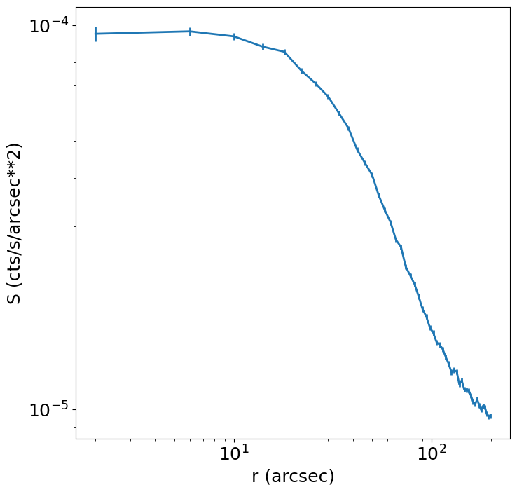
and use Matplotlib to plot some quantities. We can plot the surface brightness:

plt.figure(figsize=(8, 8))
plt.errorbar(
    f["profile"].data["rmid"],
    f["profile"].data["sur_bri"],
    lw=2,
    yerr=f["profile"].data["sur_bri_err"],
)
plt.xscale("log")
plt.yscale("log")
plt.xlabel("r (arcsec)")
plt.ylabel("S (cts/s/arcsec**2)")

Text(0, 0.5, 'S (cts/s/arcsec**2)')

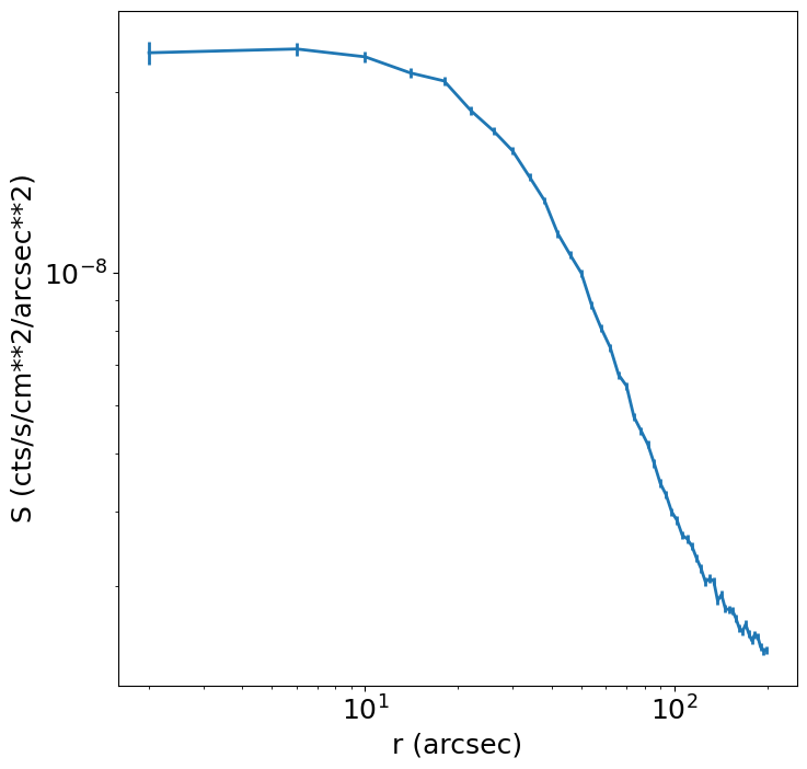
and, since we used an exposure map, the surface flux:

plt.figure(figsize=(8, 8))
plt.errorbar(
    f["profile"].data["rmid"],
    f["profile"].data["sur_flux"],
    lw=2,
    yerr=f["profile"].data["sur_flux_err"],
)
plt.xscale("log")
plt.yscale("log")
plt.xlabel("r (arcsec)")
plt.ylabel("S (cts/s/cm**2/arcsec**2)")

Text(0, 0.5, 'S (cts/s/cm**2/arcsec**2)')