X-ray Fields for yt
The simplest use of a SourceModel in pyXSIM is
to create fields of X-ray emission that can be used in yt to compute emissivities,
luminosities, or intensities. These can be computed for geometric objects such as
spheres or boxes or can be projected along a sight line. There are two methods to do
this which are described below.
Source Fields
One may want to compute fields for the emissivity or the luminosity of a particular
source in its rest/source frame. This can be done using the
make_source_fields() method. This
method takes a Dataset object from yt,
and the minimum and maximum energies of the band you want to create fields for.
The example below shows creating source fields for thermal emission from a simulation
of a galaxy cluster:
import yt
import pyxsim

ds = yt.load("GasSloshing/sloshing_nomag2_hdf5_plt_cnt_0100",
             default_species_fields="ionized")

emin = 0.1
emax = 10.0
nbins = 1000
Zmet = 0.3 # this dataset does not have a metallicity field, so assume 0.3 Zsolar
source_model = pyxsim.CIESourceModel("apec", emin, emax, nbins, Zmet)

# arguments are the Dataset, and the emin and emax of the
# band
xray_fields = source_model.make_source_fields(ds, 0.5, 7.0)
The fields are created for the Dataset
ds, and their names are returned in the xray_fields list:
print(xray_fields)
[('gas', 'xray_emissivity_0.5_7.0_keV'),
 ('gas', 'xray_luminosity_0.5_7.0_keV'),
 ('gas', 'xray_photon_emissivity_0.5_7.0_keV'),
 ('gas', 'xray_count_rate_0.5_7.0_keV')]
Four fields have been created–one for the X-ray emissivity in the chosen band in erg cm-3 s-1, another for the X-ray luminosity in the chosen band in erg s-1, another for the X-ray photon emissivity in photon cm-3 s-1, and another for the X-ray photon count rate in photon s-1. These fields exist in the same way as any other field in yt, and can be used in the same ways.
Querying emissivity values in a sphere:
sp = ds.sphere("c", (500.0, "kpc"))
print(sp['gas', 'xray_emissivity_0.5_7.0_keV'])
[6.75018212e-30 6.63582106e-30 6.45686636e-30 ... 2.59468150e-30
 2.55886161e-30 2.65063999e-30] erg/(cm**3*s)
Summing luminosity in a sphere:
print(sp.sum(("gas", "xray_luminosity_0.5_7.0_keV")))
unyt_quantity(7.73753352e+44, 'erg/s')
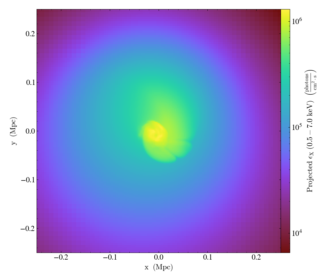
Projecting the photon emissivity along a sight line:
prj = yt.ProjectionPlot(ds, "z", xray_fields[-2], width=(0.5, "Mpc"))
prj.save()
It is possible if one desires to adjust the names for the fields that are
created using the band_name keyword argument. If specified, this argument
will replace the "{emin}_{emax}_keV part of the field name with the string
given in band_name:
xray_fields = source_model.make_source_fields(ds, 0.5, 7.0, band_name="broad")
print(xray_fields)
[('gas', 'xray_emissivity_broad'),
 ('gas', 'xray_luminosity_broad'),
 ('gas', 'xray_photon_emissivity_broad'),
 ('gas', 'xray_count_rate_broad')]
Intensity Fields
If instead one wants to compute the intensity fields in the observer frame, which
is at a given distance or redshift from the source, this can be done using the
make_intensity_fields() method. This
method takes a Dataset object from yt,
the minimum and maximum energies of the band you want to create fields for, and either
the cosmological redshift of the source (which gives the distance) or the local distance
for a nearby source. These fields are designed specifically for making projections. By
default, these fields also take into account the Doppler shifting of the individual volume
or mass elements of the source. For this reason, constructing these fields may take more
computational time.
The example below shows creating source fields for thermal emission from a simulation of the circumgalactic medium of a disk galaxy:
import yt
import pyxsim

def hot_gas(pfilter, data):
    pfilter1 = data[pfilter.filtered_type, "temperature"] > 3.0e5
    pfilter2 = data[pfilter.filtered_type, "star_formation_rate"] == 0.0
    pfilter3 = data[pfilter.filtered_type, "density"] < 3.0e-25
    return pfilter1 & pfilter2 & pfilter3

yt.add_particle_filter(
    "hot_gas",
    function=hot_gas,
    filtered_type="gas",
    requires=["temperature", "star_formation_rate", "density"],
)

ds = yt.load("cutout_37.hdf5",
             bounding_box=[[-1000.0, 1000], [-1000.0, 1000], [-1000.0, 1000]])
ds.add_particle_filter("hot_gas")

source_model = pyxsim.IGMSourceModel(
    0.2,
    3.0,
    1000,
    ("hot_gas", "metallicity"),
    binscale="log",
    resonant_scattering=False,
    cxb_factor=0.5,
    kT_max=30.0,
    nh_field=("hot_gas","H_nuclei_density"),
    temperature_field=("hot_gas", "temperature"),
    emission_measure_field=("hot_gas", "emission_measure"),
)

# arguments are the Dataset, the emin and emax of the band, and the redshift
xray_fields = source_model.make_intensity_fields(ds, 0.55, 0.65, redshift=0.01)
The fields are created for the Dataset
ds, and their names are returned in the xray_fields list:
print(xray_fields)
[('hot_gas', 'xray_intensity_0.55_0.65_keV'),
 ('hot_gas', 'xray_photon_intensity_0.55_0.65_keV')]
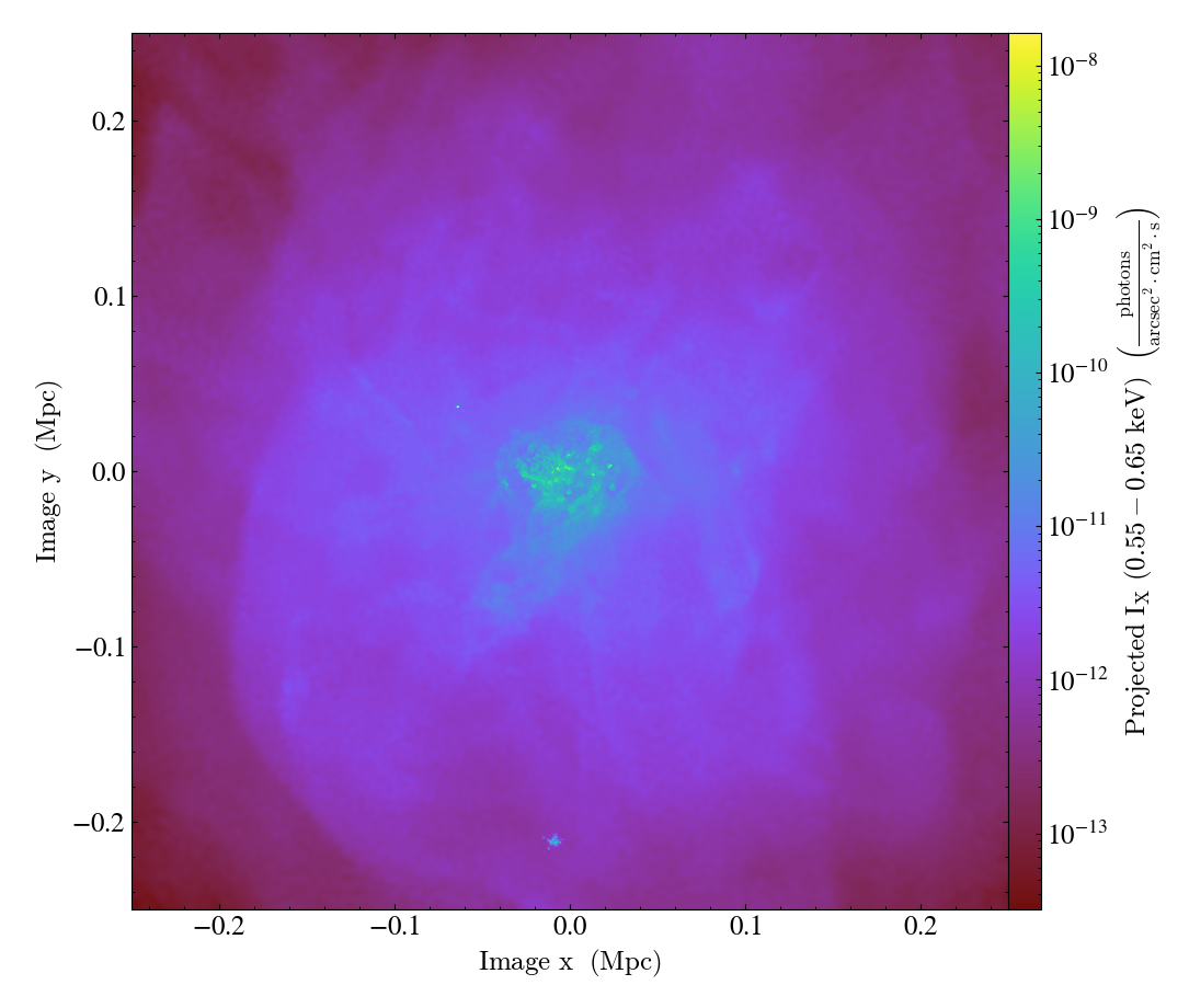
These can be used to make projections:
prj = yt.OffAxisProjectionPlot(ds, [0.0, -1.0, 1.0], xray_fields[-1],
                           width=(0.5,"Mpc"), north_vector=[0.0, 1.0, 1.0])
prj.save()
As with the source fields, it is possible to adjust the names for the fields that
are produced by passing in the band_name keyword argument.
By default, these fields are created taking into account the Doppler shifting of the
individual volume or mass elements of the source. This can be very computationally
expensive. If one does not want this, the no_doppler keyword argument can be set to True in the call to
make_intensity_fields().
Line Fields
At times it may be more convenient to specify a source or intensity field based
on a very narrow bandpass around a line centroid. For this, pyXSIM provides the
make_line_source_fields()
and make_line_intensity_fields() methods. These
are essentially just wrappers around make_source_fields()
and make_intensity_fields() which allow one
to specify a narrow bandpass around a line centroid and give it a specific name:
src_fields = source_model.make_line_source_fields(
    ds, (0.561, "keV"), (2, "eV"), "O_VII"
)
I_fields = source_model.make_line_intensity_fields(
    ds, (0.64752, "keV"), (3.0, "eV"), "O_VIII", redshift=0.01
)
Otherwise, the properties of the fields are the same as their broader counterparts.