More Advanced Thermal Emission

In this example, we’ll look at the emission from a disk galaxy from the Illustris TNG simulations. This dataset has metallicity information for several species in it. We’ll make a cut in phase space like we did in the previous example. The dataset we want to use for this example is available for download here.

First, import our necessary modules:

import yt
import pyxsim
import soxs

We will make phase space cuts on the gas cells using density, temperature, and star formation rate:

# Note that the units of all numbers in this function are CGS
# define hot gas filter
def hot_gas(pfilter, data):
    pfilter1 = data[pfilter.filtered_type, "temperature"] > 3.0e5
    pfilter2 = data["PartType0", "StarFormationRate"] == 0.0
    pfilter3 = data[pfilter.filtered_type, "density"] < 5e-25
    return pfilter1 & pfilter2 & pfilter3


yt.add_particle_filter(
    "hot_gas",
    function=hot_gas,
    filtered_type="gas",
    requires=["temperature", "density"],
)

Next, we load the dataset with yt, and add the "hot_gas" filter to the dataset:

ds = yt.load(
    "cutout_31_rotated.hdf5",
    bounding_box=[[-1000.0, 1000], [-1000.0, 1000], [-1000.0, 1000]],
)
ds.add_particle_filter("hot_gas")

yt : [INFO     ] 2025-11-06 15:48:57,356 Calculating time from 1.000e+00 to be 4.356e+17 seconds
yt : [INFO     ] 2025-11-06 15:48:57,382 Parameters: current_time              = 4.355810528213311e+17 s
yt : [INFO     ] 2025-11-06 15:48:57,383 Parameters: domain_dimensions         = [1 1 1]
yt : [INFO     ] 2025-11-06 15:48:57,383 Parameters: domain_left_edge          = [-1000. -1000. -1000.]
yt : [INFO     ] 2025-11-06 15:48:57,383 Parameters: domain_right_edge         = [1000. 1000. 1000.]
yt : [INFO     ] 2025-11-06 15:48:57,383 Parameters: cosmological_simulation   = True
yt : [INFO     ] 2025-11-06 15:48:57,384 Parameters: current_redshift          = 2.220446049250313e-16
yt : [INFO     ] 2025-11-06 15:48:57,384 Parameters: omega_lambda              = 0.6911
yt : [INFO     ] 2025-11-06 15:48:57,384 Parameters: omega_matter              = 0.3089
yt : [INFO     ] 2025-11-06 15:48:57,384 Parameters: omega_radiation           = 0.0
yt : [INFO     ] 2025-11-06 15:48:57,384 Parameters: hubble_constant           = 0.6774
yt : [WARNING  ] 2025-11-06 15:48:57,384 A bounding box was explicitly specified, so we are disabling periodicity.
yt : [INFO     ] 2025-11-06 15:48:57,414 Allocating for 2.734e+07 particles
Loading particle index: 100%|██████████████████████████████████████████████████████| 63/63 [00:00<00:00, 1286.77it/s]

True

We also need to tell pyXSIM which elements have fields in the dataset that should be used. To do this we create a var_elem dictionary of (key, value) pairs corresponding to the element name and the yt field name (assuming the "hot_gas" type).

# metal fields to use
metals = [
    "C_fraction",
    "N_fraction",
    "O_fraction",
    "Ne_fraction",
    "Mg_fraction",
    "Si_fraction",
    "Fe_fraction",
]
var_elem = {elem.split("_")[0]: ("hot_gas", elem) for elem in metals}

Now that we have everything we need, we’ll set up the IGMSourceModel, which is based on Cloudy and includes resonant scattering off of the CXB (see here for more details). Because we created a hot gas filter, we will use the "hot_gas" field type for the emission measure, temperature, and metallicity fields.

source_model = pyxsim.IGMSourceModel(
    0.1,
    4.0,
    5000,
    ("hot_gas", "metallicity"),
    binscale="log",
    resonant_scattering=True,
    temperature_field=("hot_gas", "temperature"),
    emission_measure_field=("hot_gas", "emission_measure"),
    nh_field=("hot_gas", "H_nuclei_density"),
    var_elem=var_elem,
)

pyxsim : [INFO     ] 2025-11-06 15:49:00,459 kT_min = 0.00431 keV
pyxsim : [INFO     ] 2025-11-06 15:49:00,459 kT_max = 64 keV

As in other examples, we choose big numbers for the collecting area and exposure time, and a redshift:

exp_time = (1.0, "Ms")  # exposure time
area = (5000.0, "cm**2")  # collecting area
redshift = 0.01

Next, we’ll create a box object to serve as a source for the photons. The dataset consists of only the galaxy at a specific location, which we use below, and pick a width of 1 Mpc:

c = ds.arr([0.0, 0.0, 0.0], "code_length")
width = ds.quan(1.0, "Mpc")
le = c - 0.5 * width
re = c + 0.5 * width
box = ds.box(le, re)

So, that’s everything–let’s create the photons! We use the make_photons function for this:

n_photons, n_cells = pyxsim.make_photons(
    "cutout_31_photons", box, redshift, area, exp_time, source_model
)

pyxsim : [INFO     ] 2025-11-06 15:49:00,470 Cosmology: h = 0.6774, omega_matter = 0.3089, omega_lambda = 0.6911
pyxsim : [INFO     ] 2025-11-06 15:49:00,471 Using emission measure field '('hot_gas', 'emission_measure')'.
pyxsim : [INFO     ] 2025-11-06 15:49:00,471 Using temperature field '('hot_gas', 'temperature')'.
pyxsim : [INFO     ] 2025-11-06 15:49:00,471 Using nH field '('hot_gas', 'H_nuclei_density')'.

pyxsim : [INFO     ] 2025-11-06 16:15:02,977 Finished generating photons.
pyxsim : [INFO     ] 2025-11-06 16:15:02,977 Number of photons generated: 9282882
pyxsim : [INFO     ] 2025-11-06 16:15:02,978 Number of cells with photons: 1594028

And now we create events using the project_photons function. Let’s project along the "z" axis. We’ll use the "tbabs" foreground absorption model this time, with a neutral hydrogen column of \(N_H = 2 \times 10^{20}~{\rm cm}^{-2}\):

n_events = pyxsim.project_photons(
    "cutout_31_photons",
    "cutout_31_events",
    "x",
    (30.0, 45.0),
    absorb_model="tbabs",
    nH=0.02,
)

pyxsim : [INFO     ] 2025-11-06 16:15:02,984 Foreground galactic absorption: using the tbabs model and nH = 0.02.

pyxsim : [INFO     ] 2025-11-06 16:15:04,348 Detected 1830262 events.

Now that we have a set of “events” on the sky, we can use them as an input to the instrument simulator in SOXS. We’ll observe it with the 2eV LEM model for 1 Ms. First, we’ll create a background file that we’ll use for the background:

soxs.make_background_file(
    "bkgnd_evt_31.fits", (1000.0, "ks"), "lem_2eV", [30.0, 45.0], overwrite=True
)

soxs : [INFO     ] 2025-11-06 16:15:04,499 Adding in point-source background.
soxs : [INFO     ] 2025-11-06 16:15:16,390 Simulating events from 1 sources using instrument lem_2eV for 1000 ks.
soxs : [INFO     ] 2025-11-06 16:15:19,164 Scattering energies with RMF lem_2ev_110422.rmf.

soxs : [INFO     ] 2025-11-06 16:15:28,595 Detected 3771313 events in total.
soxs : [INFO     ] 2025-11-06 16:15:28,611 Generated 3771313 photons from the point-source background.
soxs : [INFO     ] 2025-11-06 16:15:28,611 Adding in astrophysical foreground.

soxs : [INFO     ] 2025-11-06 16:15:32,267 Adding in instrumental background.
soxs : [INFO     ] 2025-11-06 16:15:32,504 Making 6280957 events from the galactic foreground.
soxs : [INFO     ] 2025-11-06 16:15:32,505 Making 3409332 events from the instrumental background.
soxs : [INFO     ] 2025-11-06 16:15:33,286 Writing background events to file bkgnd_evt_31.fits.

Now we simulate the source itself, adding in the background:

soxs.instrument_simulator(
    "cutout_31_events.h5",
    "evt_31.fits",
    (1000.0, "ks"),
    "lem_2eV",
    [30.0, 45.0],
    overwrite=True,
    bkgnd_file="bkgnd_evt_31.fits",
)

soxs : [INFO     ] 2025-11-06 16:15:34,367 Simulating events from 1 sources using instrument lem_2eV for 1000 ks.
soxs : [INFO     ] 2025-11-06 16:15:34,605 Scattering energies with RMF lem_2ev_110422.rmf.

soxs : [INFO     ] 2025-11-06 16:15:35,599 Detected 357403 events in total.
soxs : [INFO     ] 2025-11-06 16:15:35,604 Adding background events from the file bkgnd_evt_31.fits.
soxs : [INFO     ] 2025-11-06 16:15:36,571 Adding 13461602 background events from bkgnd_evt_31.fits.
soxs : [INFO     ] 2025-11-06 16:15:37,650 Observation complete.
soxs : [INFO     ] 2025-11-06 16:15:37,666 Writing events to file evt_31.fits.

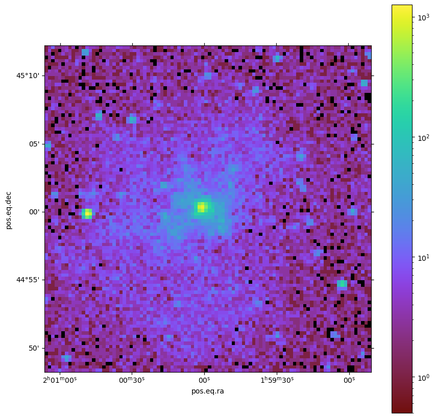
We can use the write_image() function in SOXS to bin the events into an image and write them to a file, restricting the energies between 0.644 and 0.65 keV, which focuses on the redshifted OVIII line:

soxs.write_image("evt_31.fits", "img_31.fits", emin=0.644, emax=0.65, overwrite=True)

Now we can take a quick look at the image:

soxs.plot_image("img_31.fits", stretch="log", cmap="arbre", width=0.4, vmin=0.5)

(<Figure size 1000x1000 with 2 Axes>, <WCSAxes: >)

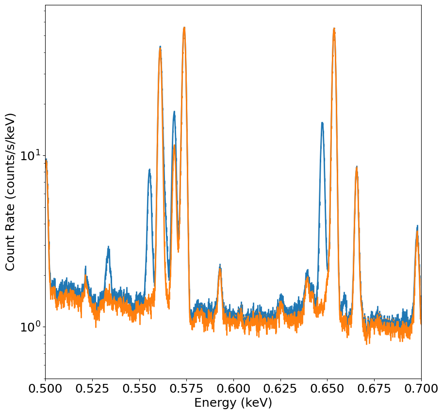
Now we will make spectra to look at. First, filter the events of both the combined source and background files and the background-only files within 0.15 degree of the center:

soxs.filter_events(
    "evt_31.fits",
    "evt_31_filter.fits",
    overwrite=True,
    region='fk5\ncircle(30.0000000,45.0000000,540.000")',
)
soxs.filter_events(
    "bkgnd_evt_31.fits",
    "bkgnd_evt_31_filter.fits",
    overwrite=True,
    region='fk5\ncircle(30.0000000,45.0000000,540.000")',
)

Now bin up spectra for these new event files:

soxs.write_spectrum("evt_31_filter.fits", "evt_31.pi", overwrite=True)
soxs.write_spectrum("bkgnd_evt_31_filter.fits", "bkgnd_evt_31.pi", overwrite=True)

Finally, we can plot the spectra. Below, the total spectrum is in blue and the background/foreground spectrum is in orange. The lines from the emission of the distant galaxy are redshifted away from the foreground Milky Way lines.

fig, ax, _ = soxs.plot_spectrum("evt_31.pi", xmin=0.5, xmax=0.7, xscale="linear", yscale="log", color="C0", ymin=0.5)
soxs.plot_spectrum("bkgnd_evt_31.pi", xmin=0.5, xmax=0.7, fig=fig, ax=ax, yscale="log", color="C1", ymin=0.5)

(<Figure size 1000x1000 with 1 Axes>,
 <Axes: xlabel='Energy (keV)', ylabel='Count Rate (counts/s/keV)'>,
 array([0.1    , 0.10025, 0.1005 , ..., 3.0995 , 3.09975, 3.1    ],
       shape=(12001,)))