“Internal” Observers and “All-Sky” Observations
The default observing mode for pyXSIM is that of an “external” observer at a very large distance from a source. In this mode, we assume a flat-sky approximation for projecting the photons. It is also possible to make observations for nearby sources for which this approximation no longer applies, and a “spherical projection” is assumed. Such sources could be a large, nearby object, or a simulation of the emission from the hot gas of a galaxy from within the galaxy itself. In these cases, the flux of photons from each part (cell or particle) of the source depends on the distance to that part of the source, as opposed to the distance to the source as a whole for the “flat-sky” case. In this mode, photons could come from sources at any position on the sky, so it is ideal for making all-sky maps.
Instead of the project_photons() function, this functionality
uses the project_photons_allsky() function, which takes the
following parameters:
photon_prefix: The prefix of the filename(s) containing the photon list. If run in serial, the filename will be “{photon_prefix}.h5”, if run in parallel, the filenames will be “{photon_prefix}.{mpi_rank}.h5”.event_prefix: The prefix of the filename(s) which will be written to contain the event list. If run in serial, the filename will be"{event_prefix}.h5", if run in parallel, the filename will be"{event_prefix}.{mpi_rank}.h5".normal: The vector determining the “z” or “up” vector for the spherical coordinate system for the all-sky projection, something like [1.0, 2.0, -3.0]absorb_model(optional): A string representing a model for foreground galactic absorption. The two models included in pyXSIM for absorption are:"wabs"(Wisconsin (Morrison and McCammon; ApJ 270, 119)), and"tbabs"(Tuebingen-Boulder (Wilms, J., Allen, A., & McCray, R. 2000, ApJ, 542, 914)). The default is no absorption–if an absorption model is chosen, thenHparameter must also be set.nH(optional): The foreground galactic column density in units of 1022 atoms cm-2, for use when one is applying foreground galactic absorption.abund_table(optional): The abundance table to be used for abundances in the TBabs absorption model. Default is set in the SOXS configuration file, the default for which is"angr". Other options are"angr","aspl","lodd","feld","wilm", and"cl17.03". For the definitions of these, see Changing the Solar Abundance Table.no_shifting(optional): If set to True, the photon energies will not be velocity Doppler shifted. Default False.center_vector(optional): A vector defining what direction will be placed at the center of the lat/lon coordinate system. If not set, an arbitrary grid-aligned center_vector perpendicular to the normal is chosen.save_los(optional): IfTrue, save the line-of-sight positions along the radial direction in units of kpc to the events list. Default:False.prng(optional): An integer seed, pseudo-random number generator,RandomStateobject, orrandom(the default). Use this if you have a reason to generate the same set of random numbers, such as for a test.
The following example shows how to create such an observation of the circumgalactic
medium from “inside a galaxy”, using a
Milky Way-sized halo
extracted from Illustris TNG (the actual dataset used is the
parent_halo with ID = 136). First, we load up the dataset in yt, and put a filter on
the gas cells so that we only consider gas that is likely to be X-ray emitting:
import yt
import numpy as np
import pyxsim
import soxs

# define hot gas filter
def hot_gas(pfilter, data):
    pfilter1 = data[pfilter.filtered_type, "temperature"] > 3.0e5
    pfilter2 = data["PartType0", "StarFormationRate"] == 0.0
    pfilter3 = data[pfilter.filtered_type, "density"] < 5e-25
    return pfilter1 & pfilter2 & pfilter3
yt.add_particle_filter("hot_gas", function=hot_gas,
                       filtered_type='gas', requires=["temperature","density"])

# load dataset and assign filter
ds = yt.load("cutout_136.hdf5")
ds.add_particle_filter("hot_gas")
Next, we specify the location of the observer and the “up” vector, which defines our coordinate system. Essentially, this determines where the “north pole” of our spherical coordinate system is.
# center of galaxy in code length
c = ds.arr([15170.3, 1034.51, 20953.5], "code_length")

# center of observer, roughly 5.4 kpc from the center of the galaxy
c_obs = c + ds.arr([3.55783736, 4.08772821, 0.], "code_length")

# "up" vector, which defines the "z" axis in a spherical coordinate
# system
L = np.array([0.71303562, -0.62060505, 0.32623548])
We want to work in the rest frame of the observer, so we compute the bulk velocity within a small sphere centered on the observer which will be used to set the frame later:
# grab a sphere of radius 0.1 kpc around the observer
s_obs = ds.sphere(c_obs, (100.0, "pc"))

# get the average gas velocity within the sphere s_obs
# use all of the gas in this case
vx = s_obs.mean(("PartType0","particle_velocity_x"), weight=("PartType0", "particle_mass"))
vy = s_obs.mean(("PartType0","particle_velocity_y"), weight=("PartType0", "particle_mass"))
vz = s_obs.mean(("PartType0","particle_velocity_z"), weight=("PartType0", "particle_mass"))
bulk_velocity = ds.arr([vx, vy, vz]).to("km/s")
Now we set up the emission model for our source:
# metal fields to use
metals = ["He_fraction", "C_fraction", "N_fraction", "O_fraction",
          "Ne_fraction", "Mg_fraction", "Si_fraction", "Fe_fraction"]
var_elem = {elem.split("_")[0]: ("hot_gas", elem) for elem in metals}

# set up the source model

emin = 0.25 # The minimum energy to generate in keV
emax = 1.5 # The maximum energy to generate in keV
nbins = 5000 # The number of energy bins between emin and emax
kT_max = 2.0 # The max gas temperature to use
source_model = pyxsim.CIESourceModel(
    "apec", emin, emax, nbins, ("hot_gas","metallicity"),
    temperature_field=("hot_gas","temperature"),
    emission_measure_field=("hot_gas", "emission_measure"),
    kT_max=kT_max, var_elem=var_elem
)
And set the observing parameters:
exp_time = (50., "s") # exposure time
area = (5000.0, "cm**2") # collecting area
redshift = 0.0 # the cosmological redshift of the source, this source is local
For determining which cells will be used in the calculation, we choose a box of 1 Mpc width centered on the center of the galaxy:
width = ds.quan(1.0, "Mpc")
le = c - 0.5*width
re = c + 0.5*width
box = ds.box(le, re)
Now we can generate the photons. We use the make_photons()
function as usual, but in this case we set observer="internal". Here, the center
is set to the observer’s location, and the bulk_velocity is set to the observer’s
velocity that we calculated above:
# make the photons
n_photons, n_cells = pyxsim.make_photons("sub_494709_photons_internal", box,
                                         redshift, area, exp_time, source_model,
                                         center=c_obs, bulk_velocity=bulk_velocity,
                                         observer="internal")
Next, we use the project_photons_allsky() function to project
the photons along all directions in a spherical projection, using L to define the
“north pole” of our sky and applying foreground Galactic absorption:
# project the photons to an all-sky map
n_events = pyxsim.project_photons_allsky("sub_494709_photons_internal",
                                         "sub_494709_events_internal", L,
                                         absorb_model="wabs", nH=0.01)
This creates a file of events that can be used as normal to create a SIMPUT catalog:
# write out the events to SIMPUT
el = pyxsim.EventList("sub_494709_events_internal.h5")
el.write_to_simput("sub_494709_events_internal", overwrite=True)
The resulting SIMPUT catalog has the same format as the case of “external” observers,
so in theory you could take any
instrument simulator that supports SIMPUT catalogs and point at
a particular location in the sky to look at it. However, it is also possible to create
an “all-sky” map with a particular instrument model using SOXS. For this, we can use
the simple_event_list() function, which simply convolves the
photons in the SIMPUT catalog with the instrument’s ARF and RMF:
# convolve the all-sky map
soxs.simple_event_list("sub_494709_events_internal_simput.fits",
                       "sub_494709_internal_evt.fits", (50.0, "s"), "lem_2eV",
                       overwrite=True, use_gal_coords=True)
No PSF scattering or any other instrumental effects are applied in this mode–the
assumption is that these effects are negligible for the angular sizes one is
investigating. The use_gal_coords=True option takes the celestial coordinates
in the file and converts them into Galactic coordinates.
The resulting event list can used to produce an “all-sky” map in X-rays using healpy like so:
import healpy as hp
import numpy as np
from astropy.io import fits
import matplotlib.pyplot as plt
# specify the minimum and maximum energies (in eV) of the band
# to plot
emin = 500.0
emax = 1500.0
# Open the file, read in the photons (making a cut on energy),
# then convert latitude and longitude to radians
with fits.open("sub_494709_internal_evt.fits") as f:
cut = (f["EVENTS"].data["ENERGY"] > emin) & (f["EVENTS"].data["ENERGY"] <= emax)
lon = np.deg2rad(f["EVENTS"].data["GLON"][cut])
lat = np.deg2rad(90.0-f["EVENTS"].data["GLAT"][cut])
# Make the histogram image using HealPy
nside = 32
pixel_indices = hp.ang2pix(nside, lat, lon)
m = np.bincount(pixel_indices, minlength=hp.nside2npix(nside))
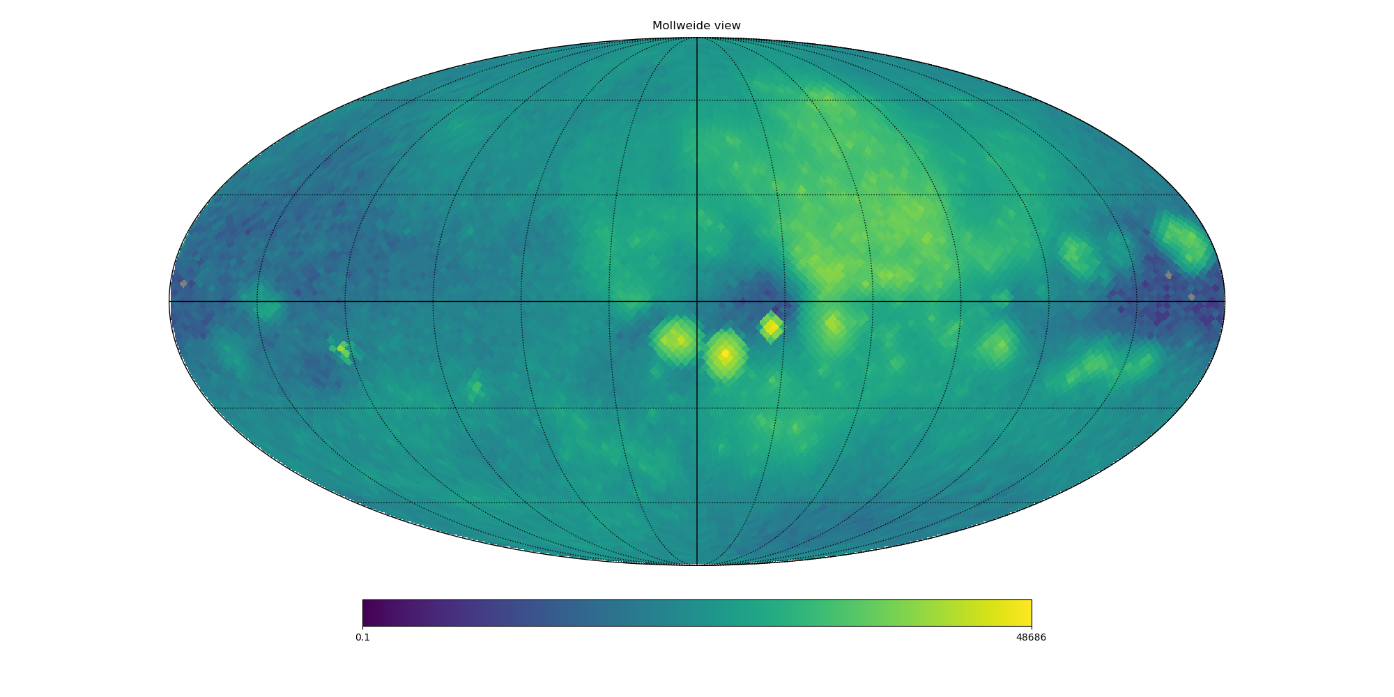
# Make a plot of the all-sky image and save
fig = plt.figure(figsize=(20,10))
hp.mollview(m, min=0.1, norm='log', fig=fig)
hp.graticule()
fig.savefig("allsky.png")
In this case, the resulting image looks like this: