Line Emission
This example shows how to create a line emission model. It uses a galaxy cluster from a Gadget SPH cosmological dataset, and will create a thermal model out of the gas particles and will use the dark matter particles to add line emission to the spectrum, assuming that the emission comes from some decay process of the dark matter.
First, we load the modules:
[1]:
%matplotlib inline
import matplotlib

matplotlib.rc("font", size=18, family="serif")
import yt
import matplotlib.pyplot as plt
from yt.units import mp
import pyxsim
As in the Advanced Thermal Emission example, we’ll set up a hot gas filter:
[2]:
# Note that the units of all numbers in this function are CGS
def hot_gas(pfilter, data):
    pfilter1 = data[pfilter.filtered_type, "density"] < 5e-25
    pfilter2 = data[pfilter.filtered_type, "temperature"] > 3481355.78432401
    pfilter3 = data[pfilter.filtered_type, "temperature"] < 4.5e8
    return (pfilter1) & (pfilter2) & (pfilter3)


yt.add_particle_filter(
    "hot_gas",
    function=hot_gas,
    filtered_type="gas",
    requires=["density", "temperature"],
)
The dataset used here does not have a field for the electron number density, which is required to construct the emission measure field. Because we’ll only be using the hot gas, we can create a ("gas","El_number_density") field which assumes complete ionization (while taking into account the H and He mass fractions vary from particle to particle). This is not strictly true for all of the "gas" type particles, but since we’ll be using the "hot_gas" type it should be sufficiently
accurate for our purposes. We’ll define the field here and add it.
[3]:
def _El_number_density(field, data):
    mueinv = data["gas", "H_fraction"] + 0.5 * (1.0 - data["gas", "He_fraction"])
    return data["gas", "density"] * mueinv / (1.0 * mp)


yt.add_field(
    ("gas", "El_number_density"),
    _El_number_density,
    units="cm**-3",
    sampling_type="local",
)
and we load the dataset in yt:
[4]:
ds = yt.load("snapshot_033/snap_033.0.hdf5")
ds.add_particle_filter("hot_gas")
yt : [INFO     ] 2026-04-13 11:27:31,925 Parameters: current_time              = 4.343952725460923e+17 s
yt : [INFO     ] 2026-04-13 11:27:31,926 Parameters: domain_dimensions         = [1 1 1]
yt : [INFO     ] 2026-04-13 11:27:31,926 Parameters: domain_left_edge          = [0. 0. 0.]
yt : [INFO     ] 2026-04-13 11:27:31,926 Parameters: domain_right_edge         = [25. 25. 25.]
yt : [INFO     ] 2026-04-13 11:27:31,927 Parameters: cosmological_simulation   = 1
yt : [INFO     ] 2026-04-13 11:27:31,927 Parameters: current_redshift          = -4.811891664902035e-05
yt : [INFO     ] 2026-04-13 11:27:31,927 Parameters: omega_lambda              = 0.762
yt : [INFO     ] 2026-04-13 11:27:31,927 Parameters: omega_matter              = 0.238
yt : [INFO     ] 2026-04-13 11:27:31,927 Parameters: omega_radiation           = 0.0
yt : [INFO     ] 2026-04-13 11:27:31,927 Parameters: hubble_constant           = 0.73
yt : [INFO     ] 2026-04-13 11:27:31,974 Allocating for 4.194e+06 particles
Loading particle index: 100%|████████████████████████████████████████████████████| 12/12 [00:00<00:00, 721.15it/s]
[4]:
True
To get a sense of what the cluster looks like, let’s take a slice through the density and temperature:
[5]:
slc = yt.SlicePlot(
    ds,
    "z",
    [("gas", "density"), ("gas", "temperature")],
    center="max",
    width=(3.0, "Mpc"),
)
slc.show()
yt : [INFO     ] 2026-04-13 11:27:32,746 max value is 7.22543e-22 at 9.1760425567626953 12.2128591537475586 9.3898868560791016
yt : [INFO     ] 2026-04-13 11:27:32,807 xlim = 8.081095 10.270990
yt : [INFO     ] 2026-04-13 11:27:32,807 ylim = 11.117912 13.307806
yt : [INFO     ] 2026-04-13 11:27:32,808 xlim = 8.081095 10.270990
yt : [INFO     ] 2026-04-13 11:27:32,809 ylim = 11.117912 13.307806
yt : [INFO     ] 2026-04-13 11:27:32,810 Making a fixed resolution buffer of (('gas', 'density')) 800 by 800
yt : [INFO     ] 2026-04-13 11:27:33,395 Making a fixed resolution buffer of (('gas', 'temperature')) 800 by 800


Now set up a sphere centered on the maximum density in the dataset:
[6]:
sp = ds.sphere("max", (1.0, "Mpc"))
yt : [INFO ] 2026-04-13 11:27:34,330 max value is 7.22543e-22 at 9.1760425567626953 12.2128591537475586 9.3898868560791016
and create a thermal source model:
[7]:
thermal_model = pyxsim.CIESourceModel("apec", 0.2, 11.0, 10000, ("gas", "metallicity"))
pyxsim : [INFO     ] 2026-04-13 11:27:34,556 kT_min = 0.025 keV
pyxsim : [INFO     ] 2026-04-13 11:27:34,556 kT_max = 64 keV
Now we’ll set up a line emission field for the dark matter particles. We won’t try to replicate a specific model, but will simply assume that the emission is proportional to the dark matter mass. Note that this field is a particle field.
[8]:
norm = yt.YTQuantity(100.0, "g**-1*s**-1")


def _dm_emission(field, data):
    return data["PartType1", "particle_mass"] * norm


ds.add_field(
    ("PartType1", "dm_emission"),
    function=_dm_emission,
    sampling_type="particle",
    units="photons/s",
    force_override=True,
)
Now we can set up the LineSourceModel object. The first argument is the line center energy in keV, and the second is the field we just created, that sets up the line amplitude. There is another parameter, sigma, for adding in broadening of the line, but in this case we’ll rely on the velocities of the dark matter particles themselves to produce the line broadening, so we’ll set this to zero.
[9]:
line_model = pyxsim.LineSourceModel(3.5, ("PartType1", "dm_emission"), (0.0, "km/s"))
Now set up the parameters for generating the photons:
[10]:
exp_time = (300.0, "ks")  # exposure time
area = (1000.0, "cm**2")  # collecting area
redshift = 0.05
and actually generate the photons:
[11]:
ntp, ntc = pyxsim.make_photons(
    "therm_photons.h5", sp, redshift, area, exp_time, thermal_model
)
nlp, nlc = pyxsim.make_photons(
    "line_photons.h5", sp, redshift, area, exp_time, line_model
)
pyxsim : [INFO     ] 2026-04-13 11:27:34,569 Cosmology: h = 0.73, omega_matter = 0.238, omega_lambda = 0.762
pyxsim : [INFO     ] 2026-04-13 11:27:34,569 Using emission measure field '('gas', 'emission_measure')'.
pyxsim : [INFO     ] 2026-04-13 11:27:34,569 Using temperature field '('gas', 'temperature')'.
pyxsim : [INFO     ] 2026-04-13 11:28:01,089 Finished generating photons.
pyxsim : [INFO     ] 2026-04-13 11:28:01,090 Number of photons generated: 1496899
pyxsim : [INFO     ] 2026-04-13 11:28:01,090 Number of cells with photons: 34544
pyxsim : [INFO     ] 2026-04-13 11:28:01,092 Cosmology: h = 0.73, omega_matter = 0.238, omega_lambda = 0.762
pyxsim : [INFO     ] 2026-04-13 11:28:01,300 Finished generating photons.
pyxsim : [INFO     ] 2026-04-13 11:28:01,301 Number of photons generated: 377
pyxsim : [INFO     ] 2026-04-13 11:28:01,301 Number of cells with photons: 376
Next, project the photons for the total set and the line set by itself:
[12]:
nte = pyxsim.project_photons(
    "therm_photons.h5",
    "therm_events.h5",
    "y",
    (30.0, 45.0),
    absorb_model="wabs",
    nH=0.02,
)
nle = pyxsim.project_photons(
    "line_photons.h5", "line_events.h5", "y", (30.0, 45.0), absorb_model="wabs", nH=0.02
)
pyxsim : [INFO ] 2026-04-13 11:28:01,306 Foreground galactic absorption: using the wabs model and nH = 0.02.
pyxsim : [INFO     ] 2026-04-13 11:28:01,492 Detected 1132648 events.
pyxsim : [INFO     ] 2026-04-13 11:28:01,493 Foreground galactic absorption: using the wabs model and nH = 0.02.
pyxsim : [INFO ] 2026-04-13 11:28:01,503 Detected 374 events.
Write the raw, unconvolved spectra to disk:
[13]:
et = pyxsim.EventList("therm_events.h5")
el = pyxsim.EventList("line_events.h5")
et.write_spectrum("therm_spec.fits", 0.1, 10.0, 5000, overwrite=True)
el.write_spectrum("line_spec.fits", 0.1, 10.0, 5000, overwrite=True)
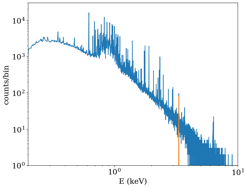
Now let’s plot up both spectra. We see that we have a thermal spectrum with the addition of a line at 3.5 keV (in real life such a line would not be so prominent, but it makes the example easier to see):
[14]:
import astropy.io.fits as pyfits

f1 = pyfits.open("therm_spec.fits")
f2 = pyfits.open("line_spec.fits")
fig = plt.figure(figsize=(9, 7))
ax = fig.add_subplot(111)
ax.loglog(
    f1["SPECTRUM"].data["ENERGY"],
    f1["SPECTRUM"].data["COUNTS"] + f2["SPECTRUM"].data["COUNTS"],
)
ax.loglog(f2["SPECTRUM"].data["ENERGY"], f2["SPECTRUM"].data["COUNTS"])
ax.set_xlim(0.2, 10)
ax.set_ylim(1, 3.0e4)
ax.set_xlabel("E (keV)")
ax.set_ylabel("counts/bin")
[14]:
Text(0, 0.5, 'counts/bin')
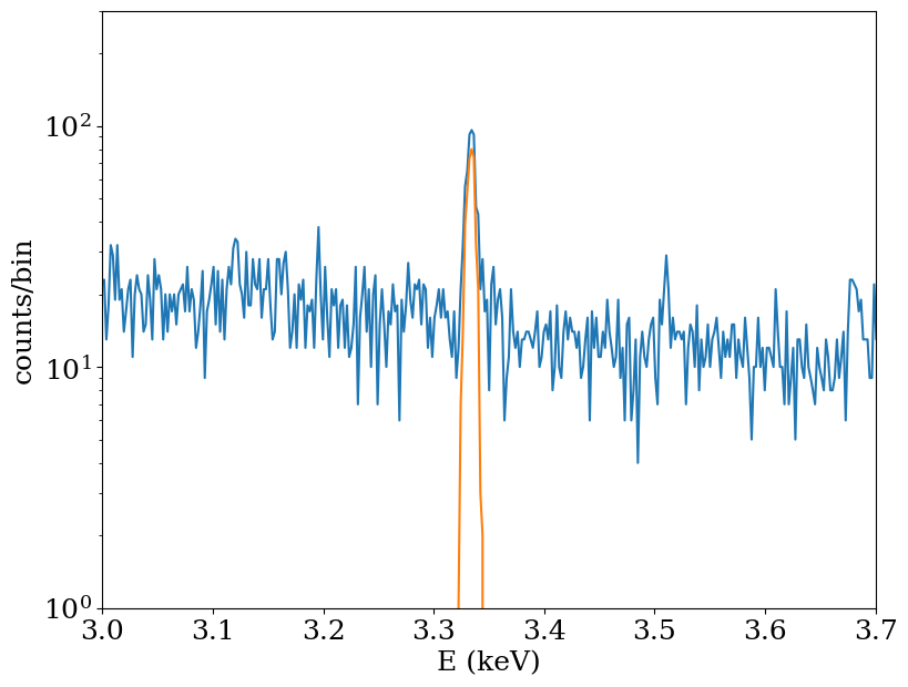
Let’s zoom into the region surrounding the line, seeing that it has some broadening due to the random velocities of the dark matter particles:
[15]:
ax.set_xscale("linear")
ax.set_xlim(3, 3.7)
ax.set_ylim(1.0, 3.0e2)
fig
[15]: