Advanced Thermal Emission
In this example, we’ll look at another galaxy cluster, but this time the dataset will have metallicity information for several species in it. In contrast to the thermal emission example, which used a grid-based dataset, the dataset we’ll use here is SPH, taken from the Magneticum suite of simulations. Finally, there are phases of gas in this dataset that will not emit in X-rays, so we also show how to make cuts in phase space and focus only on the X-ray emitting gas. The dataset we want to use for this example is available for download from the yt Project at this link.
First, import our necessary modules:
[1]:
import yt
import pyxsim
import soxs
from yt.units import mp
We mentioned above that we wanted to make phase spaces cuts on the gas. Because this is an SPH dataset, the best way to do that is with a “particle filter” in yt.
[2]:
# Note that the units of all numbers in this function are CGS
def hot_gas(pfilter, data):
    pfilter1 = data[pfilter.filtered_type, "density"] < 5e-25
    pfilter2 = data[pfilter.filtered_type, "temperature"] > 3481355.78432401
    pfilter3 = data[pfilter.filtered_type, "temperature"] < 4.5e8
    return (pfilter1) & (pfilter2) & (pfilter3)


yt.add_particle_filter(
    "hot_gas",
    function=hot_gas,
    filtered_type="gas",
    requires=["density", "temperature"],
)
The Magneticum dataset used here does not have a field for the electron number density, which is required to construct the emission measure field. Because we’ll only be using the hot gas, we can create a ("gas","El_number_density") field which assumes complete ionization (while taking into account the H and He mass fractions vary from particle to particle). This is not strictly true for all of the "gas" type particles, but since we’ll be using the "hot_gas" type it should be
sufficiently accurate for our purposes. We’ll define the field here and add it.
[3]:
def _El_number_density(field, data):
    mueinv = data["gas", "H_fraction"] + 0.5 * data["gas", "He_fraction"]
    return data["gas", "density"] * mueinv / (1.0 * mp)


yt.add_field(
    ("gas", "El_number_density"),
    _El_number_density,
    units="cm**-3",
    sampling_type="local",
)
As mentioned above, a number of elements are tracked in the SPH particles in the dataset (10 to be precise, along with a trace field for the remaining, unspecified metals). We will deal with these elements later, since we want to use the specific mass fractions of these elements to determine their emission line strengths in the mock observation. However, we also need to specify the metallicity for the rest of the (non-hydrogen) elements. The best way to do this is to sum the masses for the
metals over every particle and divide by the mass of the particle to get the metallicity for that particle. That will be assumed to be the metallicity for all non-tracked metals in this pyXSIM run. The field in the Magneticum dataset to do this is called ("Gas", "ElevenMetalMasses"), which has a shape of (number of SPH particles, 11). We’ll define this field here and add it to the dataset specifically later:
[4]:
def _metallicity(field, data):
    # We index the array starting with 1 here because the first element is
    # helium (thus not a metal)
    return data["Gas", "ElevenMetalMasses"][:, 1:].sum(axis=1) / data["Gas", "Mass"]
Next, we load the dataset with yt:
[5]:
ds = yt.load(
    "MagneticumCluster/snap_132", long_ids=True, field_spec="magneticum_box2_hr"
)
yt : [INFO     ] 2026-04-13 09:33:02,464 Calculating time from 9.081e-01 to be 3.929e+17 seconds
yt : [INFO     ] 2026-04-13 09:33:02,465 Assuming length units are in kpc/h (comoving)
yt : [INFO     ] 2026-04-13 09:33:02,489 Parameters: current_time              = 3.928659138392927e+17 s
yt : [INFO     ] 2026-04-13 09:33:02,489 Parameters: domain_dimensions         = [1 1 1]
yt : [INFO     ] 2026-04-13 09:33:02,490 Parameters: domain_left_edge          = [0. 0. 0.]
yt : [INFO     ] 2026-04-13 09:33:02,490 Parameters: domain_right_edge         = [352000. 352000. 352000.]
yt : [INFO     ] 2026-04-13 09:33:02,490 Parameters: cosmological_simulation   = True
yt : [INFO     ] 2026-04-13 09:33:02,490 Parameters: current_redshift          = 0.10114286171886899
yt : [INFO     ] 2026-04-13 09:33:02,490 Parameters: omega_lambda              = 0.728
yt : [INFO     ] 2026-04-13 09:33:02,491 Parameters: omega_matter              = 0.272
yt : [INFO     ] 2026-04-13 09:33:02,491 Parameters: omega_radiation           = 0.0
yt : [INFO     ] 2026-04-13 09:33:02,491 Parameters: hubble_constant           = 0.704
and now we add the derived fields and the "hot_gas" particle filter to this dataset. Note that for the derived fields to be picked up by the filter, they must be specified first:
[6]:
ds.add_field(("gas", "metallicity"), _metallicity, units="", sampling_type="local")
ds.add_particle_filter("hot_gas")
yt : [INFO     ] 2026-04-13 09:33:02,499 Allocating for 3.718e+06 particles
Loading particle index: 100%|█████████████████████████████████████████████████████| 6/6 [00:00<00:00, 2616.53it/s]
Loading particle index: 100%|█████████████████████████████████████████████████████| 6/6 [00:00<00:00, 7605.27it/s]
[6]:
True
We also need to tell pyXSIM which elements have fields in the dataset that should be used. To do this we create a var_elem dictionary of (key, value) pairs corresponding to the element name and the yt field name (assuming the "hot_gas" type).
[7]:
var_elem = {
    elem: ("hot_gas", f"{elem}_fraction")
    for elem in ["He", "C", "Ca", "O", "N", "Ne", "Mg", "S", "Si", "Fe"]
}
Now that we have everything we need, we’ll set up the CIESourceModel. Because we created a hot gas filter, we will use the "hot_gas" field type for the emission measure, temperature, and metallicity fields.
[8]:
source_model = pyxsim.CIESourceModel(
    "apec",
    0.1,
    10.0,
    1000,
    ("hot_gas", "metallicity"),
    temperature_field=("hot_gas", "temperature"),
    emission_measure_field=("hot_gas", "emission_measure"),
    var_elem=var_elem,
)
pyxsim : [INFO     ] 2026-04-13 09:33:03,135 kT_min = 0.025 keV
pyxsim : [INFO     ] 2026-04-13 09:33:03,135 kT_max = 64 keV
As before, we choose big numbers for the collecting area and exposure time, but the redshift should be taken from the cluster itself, since this dataset has a redshift:
[9]:
exp_time = (300.0, "ks")  # exposure time
area = (1000.0, "cm**2")  # collecting area
redshift = ds.current_redshift
Next, we’ll create a box object to serve as a source for the photons. The dataset consists of only the galaxy cluster at a specific location, which we use below, and pick a width of 3 Mpc:
[10]:
c = ds.arr([310306.53, 340613.47, 265758.47], "code_length")
width = ds.quan(3.0, "Mpc")
le = c - 0.5 * width
re = c + 0.5 * width
box = ds.box(le, re)
So, that’s everything–let’s create the photons! We use the make_photons function for this:
[11]:
n_photons, n_cells = pyxsim.make_photons(
    "snap_132_photons", box, redshift, area, exp_time, source_model
)
pyxsim : [INFO     ] 2026-04-13 09:33:03,145 Cosmology: h = 0.704, omega_matter = 0.272, omega_lambda = 0.728
pyxsim : [INFO     ] 2026-04-13 09:33:03,145 Using emission measure field '('hot_gas', 'emission_measure')'.
pyxsim : [INFO     ] 2026-04-13 09:33:03,146 Using temperature field '('hot_gas', 'temperature')'.
pyxsim : [INFO     ] 2026-04-13 09:33:26,208 Finished generating photons.
pyxsim : [INFO     ] 2026-04-13 09:33:26,218 Number of photons generated: 12618718
pyxsim : [INFO     ] 2026-04-13 09:33:26,228 Number of cells with photons: 614501
And now we create events using the project_photons function. Let’s pick an off-axis normal vector, and a north_vector to decide which way is “up.” We’ll use the "wabs" foreground absorption model this time, with a neutral hydrogen column of \(N_H = 10^{20}~{\rm cm}^{-2}\):
[12]:
L = [0.1, 0.2, -0.3]  # normal vector
N = [0.0, 1.0, 0.0]  # north vector
n_events = pyxsim.project_photons(
    "snap_132_photons",
    "snap_132_events",
    L,
    (45.0, 30.0),
    absorb_model="wabs",
    nH=0.01,
    north_vector=N,
)
pyxsim : [INFO ] 2026-04-13 09:33:26,331 Foreground galactic absorption: using the wabs model and nH = 0.01.
pyxsim : [INFO ] 2026-04-13 09:33:28,142 Detected 8584754 events.
Now that we have a set of “events” on the sky, we can read them in and write them to a SIMPUT file:
Now that we have a set of “events” on the sky, we can use them as an input to the instrument simulator in SOXS. We’ll use a small exposure time (100 ks instead of 300 ks), and observe it with the as-launched ACIS-I model:
[13]:
soxs.instrument_simulator(
    "snap_132_events.h5",
    "evt.fits",
    (100.0, "ks"),
    "chandra_acisi_cy0",
    [45.0, 30.0],
    overwrite=True,
)
soxs : [INFO     ] 2026-04-13 09:33:28,224 Simulating events from 1 sources using instrument chandra_acisi_cy0 for 100 ks.
soxs : [INFO     ] 2026-04-13 09:33:28,861 Scattering energies with RMF acisi_aimpt_cy0.rmf.
soxs : [INFO     ] 2026-04-13 09:33:29,046 Detected 495058 events in total.
soxs : [INFO     ] 2026-04-13 09:33:29,050 Adding background events.
soxs : [INFO     ] 2026-04-13 09:33:29,074 Adding in point-source background.
soxs : [INFO     ] 2026-04-13 09:33:29,578 Simulating events from 1 sources using instrument chandra_acisi_cy0 for 100 ks.
soxs : [INFO     ] 2026-04-13 09:33:29,612 Scattering energies with RMF acisi_aimpt_cy0.rmf.
soxs : [INFO     ] 2026-04-13 09:33:29,682 Detected 13299 events in total.
soxs : [INFO     ] 2026-04-13 09:33:29,683 Generated 13299 photons from the point-source background.
soxs : [INFO     ] 2026-04-13 09:33:29,683 Adding in astrophysical foreground.
soxs : [INFO     ] 2026-04-13 09:33:30,228 Adding in instrumental background.
soxs : [INFO     ] 2026-04-13 09:33:30,258 Making 6198 events from the galactic foreground.
soxs : [INFO     ] 2026-04-13 09:33:30,259 Making 126945 events from the instrumental background.
soxs : [INFO     ] 2026-04-13 09:33:30,322 Observation complete.
soxs : [INFO     ] 2026-04-13 09:33:30,323 Writing events to file evt.fits.
We can use the write_image() function in SOXS to bin the events into an image and write them to a file, restricting the energies between 0.5 and 2.0 keV:
[14]:
soxs.write_image("evt.fits", "img.fits", emin=0.5, emax=2.0, overwrite=True)
Now we can take a quick look at the image:
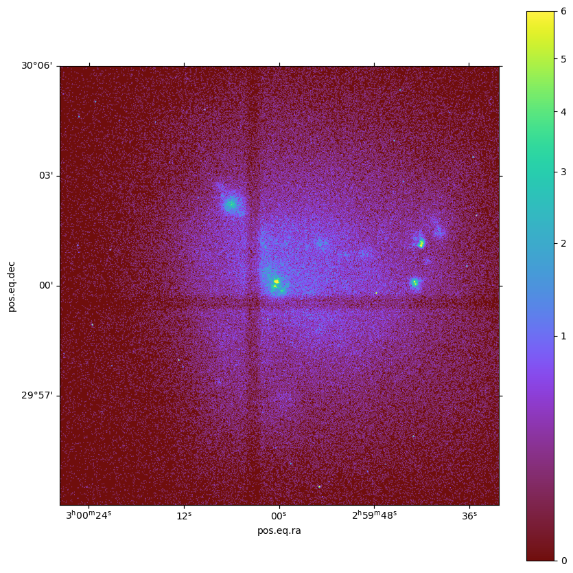
[15]:
soxs.plot_image("img.fits", stretch="sqrt", cmap="arbre", vmin=0.0, vmax=6.0, width=0.2)
[15]:
(<Figure size 1000x1000 with 2 Axes>, <WCSAxes: >)