Overview of pyXSIM’s Photon Lists
The Heritage of pyXSIM’s Photon Lists
The photon list capability in pyXSIM is an independent implementation of the PHOX algorithm, developed for constructing mock X-ray observations from SPH datasets by Veronica Biffi and Klaus Dolag. There are two relevant papers:
Biffi, V., Dolag, K., Bohringer, H., & Lemson, G. 2012, MNRAS, 420, 3545
Biffi, V., Dolag, K., Bohringer, H. 2013, MNRAS, 428, 1395
pyXSIM had a previous life as the photon_simulator analysis module as a part
of the yt Project. pyXSIM still depends critically on
yt to provide the link between the simulation data and the algorithm for
generating the X-ray photons. For detailed information about the design of the
algorithm in yt, check out
the SciPy 2014 Proceedings.
How Photon Lists Work
This section details in brief the model, assumptions, and basic algorithms of pyXSIM’s photon lists in terms of three basic steps.
Step 1: Generate Photons
We begin with a three-dimensional model of a source, whether from a dataset from some type of dynamical simulation or from a dataset constructed by hand. This dataset is comprised of cells or particles, and is understandable by yt. Examples of this may be:
A model of a galaxy cluster plasma, where the emission arises from various interactions between the thermal electrons and ions
A model of relativistic particles which emit inverse-Compton emission in a power-law spectrum
A model of dark matter particles where line emission arises from annihilation or decay of the particles
In any case, there is a fair amount of flexibility in the type of source and its emission that can be modeled. The basic idea is that for each cell or particle in a specified region of the source, photons are generated assuming the physical properties of the call and an emission model for X-rays based on those physical properties. The number of photons to be generated is controlled by specifying a fiducial exposure time, collecting area, and redshift and/or distance to the source. Typically, at this stage the values of these parameters are chosen such that they generate a large number of photons, much larger than would be actually observed, since the goal is to create an initial distribution that will be a statistically robust sample from which to draw events when creating synthetic observations. The photons are generated with three-dimensional positions in the rest frame of the source (except that their energies are potentially cosmologically redshifted with the given redshift, if the source is cosmologically distant), since the positions on the sky and the Doppler shifting of the photons are taken into account in the next step when a line of sight is provided.
Figure 1 shows a schematic example of a three-dimensional source and how the photons are generated from it. The details of how photons are created can be found in Generating Photon Lists.
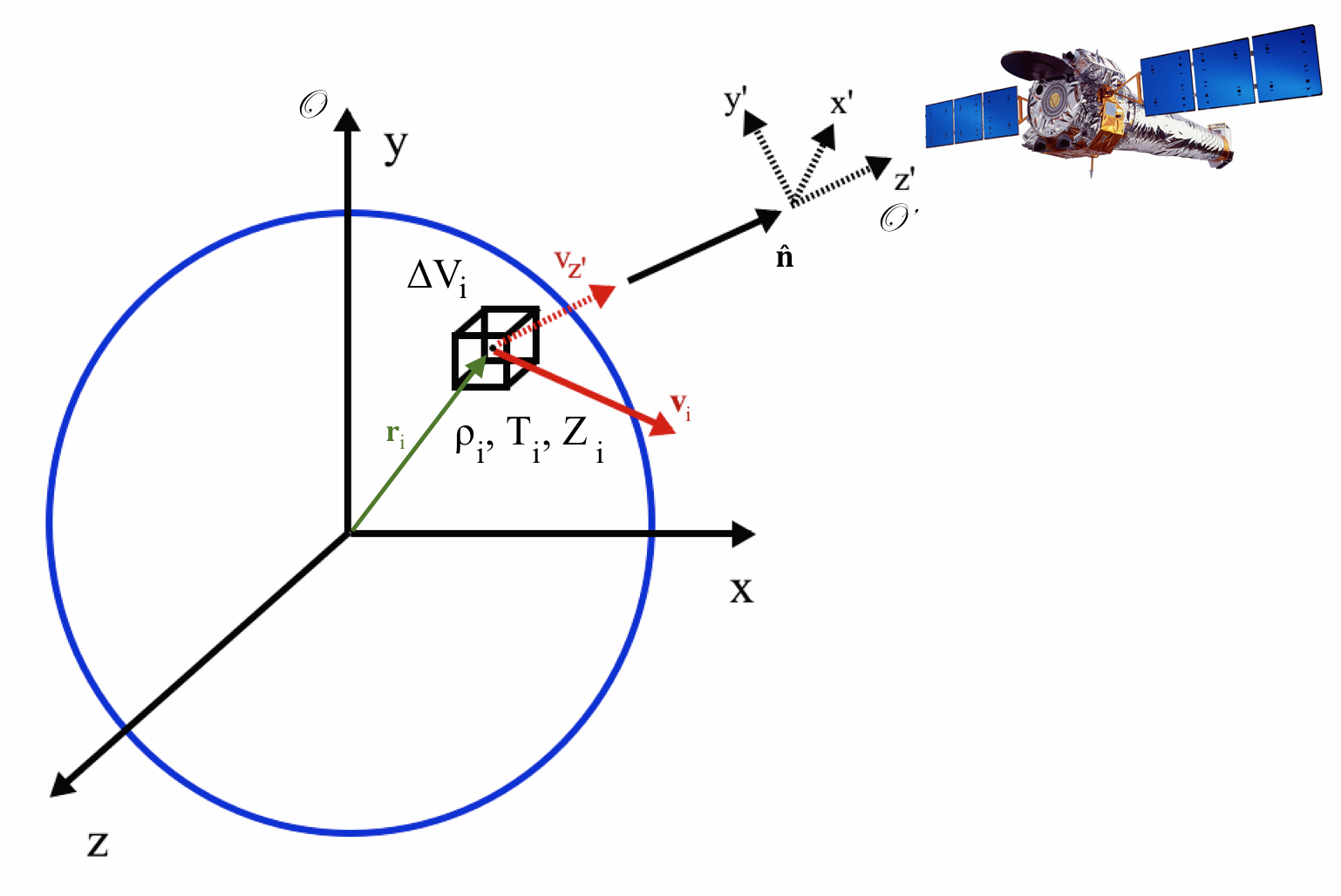
Figure 1: Schematic representation of a roughly spherical X-ray emitting object, such as a galaxy cluster. The volume element \(\Delta{V}_i\) at position \({\bf r}_i\) in the coordinate system \({\cal O}\) of the source has a velocity \({\bf v}_i\). Photons emitted along the direction given by \(\hat{\bf n}\) will be received in the observer’s frame in the coordinate system \({\cal O}'\), and will be Doppler-shifted by the line-of-sight velocity component \(v_{i,z'}\). \({\rm Chandra}\) telescope image credit: NASA/CXC.
Step 2: Project Photons to Create Events
Once we have generated our large sample of photons in the previous step, we can create a set of simulated events by projecting them along a particular line of sight. The line of sight is used to determine both the position of each event on the sky as well as the Doppler shift of the photon from the velocity of the material it was emitted from. Additionally, this is the step where foreground Galactic absorption is optionally applied. The final product is a set of events.
Figure 1 also shows how the photons are projected from the three-dimensional source along the sight-line toward the observer. The details of how events are created can be found in Event Lists.
Step 3: Convolve Events with Instrumental Responses
Finally, the last step is to take the sky-projected event positions and energies and convolve them with instrumental responses to produce realistic images and spectra that can be processed with standard software tools for working with X-ray observations. pyXSIM provides a way to export the simulated events for use with other packages which simulate X-ray observatories more accurately. The details on how to do this can be found in Producing Realistic Observations Using External Packages.