Power Law

The second example shows how to set up a power-law spectral source, as well as how to add two sets of photons together. It also shows how to use the make_spectrum functionality of a source model.

This example will also briefly show how to set up a mock dataset “in memory” using yt. For more details on how to do this, check out the yt docs on in-memory datasets.

Load up the necessary modules:

import matplotlib

matplotlib.rc("font", size=18, family="serif")
import yt
import numpy as np
import matplotlib.pyplot as plt
from yt.units import mp, keV, kpc
import pyxsim

The cluster we set up will be a simple isothermal \(\beta\)-model system, with a temperature of 4 keV. We’ll set it up on a uniform grid of 2 Mpc and 256 cells on a side. The parameters of the model are:

R = 1000.0  # radius of cluster in kpc
r_c = 100.0  # scale radius of cluster in kpc
rho_c = 1.673e-26  # scale density in g/cm^3
beta = 1.0  # beta parameter
kT = 4.0  # cluster temperature in keV
nx = 256
ddims = (nx, nx, nx)

and we set up the density and temperature arrays:

x, y, z = np.mgrid[-R : R : nx * 1j, -R : R : nx * 1j, -R : R : nx * 1j]
r = np.sqrt(x**2 + y**2 + z**2)

dens = np.zeros(ddims)
dens[r <= R] = rho_c * (1.0 + (r[r <= R] / r_c) ** 2) ** (-1.5 * beta)
dens[r > R] = 0.0
temp = (kT * keV).to_value("K", "thermal") * np.ones(ddims)

Next, we will take the density and temperature arrays and put them into a dictionary with their units, where we will also set up velocity fields set to zero. Then, we’ll call the yt function load_uniform_grid to set this up as a full-fledged yt dataset.

data = {}
data["density"] = (dens, "g/cm**3")
data["temperature"] = (temp, "K")
data["velocity_x"] = (np.zeros(ddims), "cm/s")
data["velocity_y"] = (np.zeros(ddims), "cm/s")
data["velocity_z"] = (np.zeros(ddims), "cm/s")

bbox = np.array(
    [[-0.5, 0.5], [-0.5, 0.5], [-0.5, 0.5]]
)  # The bounding box of the domain in code units

L = (2.0 * R * kpc).to_value("cm")

# We have to set default_species_fields="ionized" because
# we didn't create any species fields above
ds = yt.load_uniform_grid(data, ddims, L, bbox=bbox, default_species_fields="ionized")

yt : [INFO     ] 2024-10-07 13:34:10,037 Parameters: current_time              = 0.0
yt : [INFO     ] 2024-10-07 13:34:10,038 Parameters: domain_dimensions         = [256 256 256]
yt : [INFO     ] 2024-10-07 13:34:10,038 Parameters: domain_left_edge          = [-0.5 -0.5 -0.5]
yt : [INFO     ] 2024-10-07 13:34:10,039 Parameters: domain_right_edge         = [0.5 0.5 0.5]
yt : [INFO     ] 2024-10-07 13:34:10,039 Parameters: cosmological_simulation   = 0

The next thing we have to do is specify a derived field for the normalization of the power-law emission. This could come from a variety of sources, for example, relativistic cosmic-ray electrons. For simplicity, we’re not going to assume a specific model, except that we will only specify that the source of the power law emission is proportional to the gas mass in each cell:

norm = yt.YTQuantity(1.0e-19, "photons/s/keV")


def _power_law_emission(field, data):
    return norm * data["cell_mass"] / (1.0 * mp)


ds.add_field(
    ("gas", "power_law_emission"),
    function=_power_law_emission,
    sampling_type="local",
    units="photons/s/keV",
)

where we have normalized the field arbitrarily. Note that the emission field for a power-law model is a bit odd in that it is technically a specific luminosity for the cell. This is done primarily for simplicity in designing the underlying algorithm.

Now, let’s set up a sphere to collect photons from:

sp = ds.sphere("c", (0.5, "Mpc"))

And set the parameters for the initial photon sample:

A = yt.YTQuantity(500.0, "cm**2")
exp_time = yt.YTQuantity(1.0e5, "s")
redshift = 0.03

Set up two source models, a thermal model and a power-law model:

therm_model = pyxsim.CIESourceModel("apec", 1, 80.0, 5000, Zmet=0.3)
plaw_model = pyxsim.PowerLawSourceModel(1.0, 1, 80.0, "power_law_emission", 1.0)

pyxsim : [INFO     ] 2024-10-07 13:34:10,500 kT_min = 0.025 keV
pyxsim : [INFO     ] 2024-10-07 13:34:10,500 kT_max = 64 keV

Now, generate the photons for each source model:

ntp, ntc = pyxsim.make_photons("therm_photons", sp, redshift, A, exp_time, therm_model)
npp, npc = pyxsim.make_photons("plaw_photons", sp, redshift, A, exp_time, plaw_model)

pyxsim : [INFO     ] 2024-10-07 13:34:10,510 Cosmology: h = 0.71, omega_matter = 0.27, omega_lambda = 0.73
pyxsim : [INFO     ] 2024-10-07 13:34:10,510 Using emission measure field '('gas', 'emission_measure')'.
pyxsim : [INFO     ] 2024-10-07 13:34:10,510 Using temperature field '('gas', 'temperature')'.

pyxsim : [INFO     ] 2024-10-07 13:35:22,671 Finished generating photons.
pyxsim : [INFO     ] 2024-10-07 13:35:22,677 Number of photons generated: 336467
pyxsim : [INFO     ] 2024-10-07 13:35:22,678 Number of cells with photons: 93402
pyxsim : [INFO     ] 2024-10-07 13:35:22,689 Cosmology: h = 0.71, omega_matter = 0.27, omega_lambda = 0.73
pyxsim : [INFO     ] 2024-10-07 13:35:23,200 Finished generating photons.
pyxsim : [INFO     ] 2024-10-07 13:35:23,201 Number of photons generated: 54184
pyxsim : [INFO     ] 2024-10-07 13:35:23,201 Number of cells with photons: 49091

Now, we want to project the photons along a line of sight. We’ll specify the "wabs" model for foreground galactic absorption. We’ll create events from the total set of photons as well as the power-law only set, to see the difference between the two.

nte = pyxsim.project_photons(
    "therm_photons", "therm_events", "x", (30.0, 45.0), absorb_model="wabs", nH=0.02
)
npe = pyxsim.project_photons(
    "plaw_photons", "plaw_events", "x", (30.0, 45.0), absorb_model="wabs", nH=0.02
)

pyxsim : [INFO     ] 2024-10-07 13:35:23,210 Foreground galactic absorption: using the wabs model and nH = 0.02.

pyxsim : [INFO     ] 2024-10-07 13:35:23,298 Detected 331602 events.
pyxsim : [INFO     ] 2024-10-07 13:35:23,302 Foreground galactic absorption: using the wabs model and nH = 0.02.

pyxsim : [INFO     ] 2024-10-07 13:35:23,331 Detected 53942 events.

Finally, create energy spectra for both sets of events. We won’t bother convolving with instrument responses here, because we just want to see what the spectra look like.

et = pyxsim.EventList("therm_events.h5")
ep = pyxsim.EventList("plaw_events.h5")
et.write_spectrum("therm_spec.fits", 1, 80.0, 5000, overwrite=True)
ep.write_spectrum("plaw_spec.fits", 1, 80.0, 5000, overwrite=True)

To visualize the spectra, we’ll load them up using AstroPy’s FITS I/O and use Matplotlib to plot the spectra:

import astropy.io.fits as pyfits

f1 = pyfits.open("therm_spec.fits")
f2 = pyfits.open("plaw_spec.fits")
plt.figure(figsize=(9, 7))
plt.loglog(
    f2["SPECTRUM"].data["ENERGY"], f2["SPECTRUM"].data["COUNTS"], label="Power-Law"
)
plt.loglog(
    f2["SPECTRUM"].data["ENERGY"],
    f1["SPECTRUM"].data["COUNTS"] + f2["SPECTRUM"].data["COUNTS"],
    label="Power-Law+Thermal",
)
plt.xlim(1, 50)
plt.ylim(1, 2.0e4)
plt.legend()
plt.xlabel("E (keV)")
plt.ylabel("counts/bin")

Text(0, 0.5, 'counts/bin')

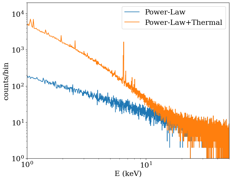
As you can see, the orange line shows a sum of a thermal and power-law spectrum, the latter most prominent at high energies. The blue line shows the power-law spectrum. Both spectra are absorbed at low energies, thanks to the Galactic foreground absorption.

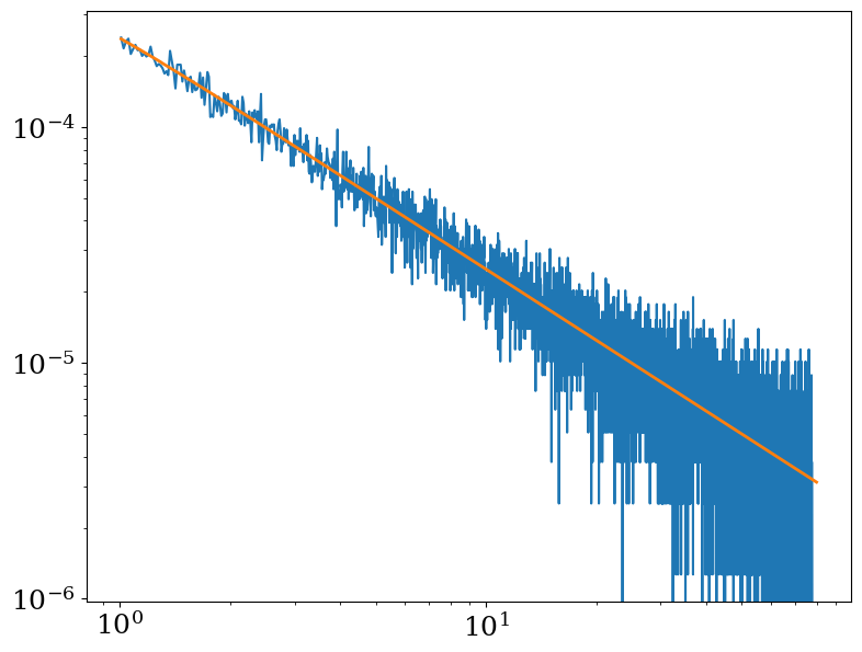
Finally, we show how to make a spectrum of the entire sphere object using the make_spectrum method of the PowerLawSourceModel. To do this, we simply supply make_spectrum with the sphere object, the minimum and maximum energies in the spectrum, the number of bins in the spectrum, and optionally the redshift. The latter ensures we get a flux spectrum in the observer frame. make_spectrum returns a SOXS Spectrum object, which you can do other things with, such as apply foreground absorption.

emin = 1.0
emax = 80.0
nbins = 5000
pspec = plaw_model.make_spectrum(sp, emin, emax, nbins, redshift=redshift)
pspec.apply_foreground_absorption(0.02)

To show this is the same spectrum that we obtained above, we compare it to the above spectrum we derived from the mock photons we generated before (converting it to a flux first).

emid = f2["SPECTRUM"].data["ENERGY"]
de = np.diff(emid)[0]
# We have to convert counts/bin to counts/s/cm**2/keV here
flux = f2["SPECTRUM"].data["COUNTS"] / (A.v * exp_time.v * de)
plt.figure(figsize=(9, 7))
plt.loglog(emid, flux)
plt.loglog(pspec.emid, pspec.flux, lw=2)

[<matplotlib.lines.Line2D at 0x1667f60c0>]