Thermal Emission

The first example we’ll look at is that of thermal emission from a galaxy cluster. In this case, the gas in the core of the cluster is “sloshing” in the center, producing spiral-shaped cold fronts. The dataset we want to use for this example is available for download from the yt Project at this link.

First, import our necessary modules:

import yt
import pyxsim
import soxs

Next, we load the dataset with yt. Note that this dataset does not have species fields in it, so we’ll set default_species_fields="ionized" to assume full ionization (as appropriate for galaxy clusters):

ds = yt.load(
    "GasSloshing/sloshing_nomag2_hdf5_plt_cnt_0150", default_species_fields="ionized"
)

yt : [INFO     ] 2026-04-13 10:15:46,629 Parameters: current_time              = 1.1835090993823291e+17
yt : [INFO     ] 2026-04-13 10:15:46,629 Parameters: domain_dimensions         = [16 16 16]
yt : [INFO     ] 2026-04-13 10:15:46,630 Parameters: domain_left_edge          = [-3.70272e+24 -3.70272e+24 -3.70272e+24]
yt : [INFO     ] 2026-04-13 10:15:46,630 Parameters: domain_right_edge         = [3.70272e+24 3.70272e+24 3.70272e+24]
yt : [INFO     ] 2026-04-13 10:15:46,630 Parameters: cosmological_simulation   = 0

Let’s use yt to take a slice of density and temperature through the center of the dataset so we can see what we’re looking at, as well as overplotting velocity vectors to see the sloshing motion of the gas:

slc = yt.SlicePlot(
    ds, "z", [("gas", "density"), ("gas", "temperature")], width=(1.0, "Mpc")
)
slc.annotate_velocity()

yt : [INFO     ] 2026-04-13 10:15:46,943 xlim = -1542838790481162406985728.000000 1542838790481162406985728.000000
yt : [INFO     ] 2026-04-13 10:15:46,944 ylim = -1542838790481162406985728.000000 1542838790481162406985728.000000
yt : [INFO     ] 2026-04-13 10:15:46,945 xlim = -1542838790481162406985728.000000 1542838790481162406985728.000000
yt : [INFO     ] 2026-04-13 10:15:46,945 ylim = -1542838790481162406985728.000000 1542838790481162406985728.000000
yt : [INFO     ] 2026-04-13 10:15:46,948 Making a fixed resolution buffer of (('gas', 'density')) 800 by 800
yt : [INFO     ] 2026-04-13 10:15:47,160 Making a fixed resolution buffer of (('gas', 'temperature')) 800 by 800

Ok, sloshing gas as advertised. Next, we’ll create a sphere object to serve as a source for some of our investigations. Place it at the center of the domain with "c", and use a radius of 500 kpc:

sp = ds.sphere("c", (500.0, "kpc"))

Now, we need to set up a source model. We said we were going to look at the thermal emission from the hot plasma, which in a galaxy cluster is in collisional ionization equilibrium (CIE), so to do that we can set up a CIESourceModel. The first argument specifies which model we want to use. Let’s use "spex". The next three arguments are the maximum and minimum energies, and the number of bins in the spectrum. We’ve chosen these numbers so that the spectrum has an energy resolution of about 1.25 eV.

CIESourceModel takes a lot of optional arguments, which you can investigate in the docs, but here we’ll do something simple and say that the metallicity is a constant \(Z = 0.3~Z_\odot\) (since there are no metal fields in this source):

source_model = pyxsim.CIESourceModel("spex", 0.2, 9.0, 7000, 0.3, binscale="log")

pyxsim : [INFO     ] 2026-04-13 10:15:48,104 kT_min = 0.025 keV
pyxsim : [INFO     ] 2026-04-13 10:15:48,105 kT_max = 64 keV

Creating Emission Fields

We can use this source_model object to compute X-ray fields for use in calculations. For example, we can create fields for emissivity, luminosity, and photon emissivity within a particular band, in this case 0.5-7 keV:

xray_fields = source_model.make_source_fields(ds, 0.5, 7.0)
print(xray_fields)

pyxsim : [INFO     ] 2026-04-13 10:15:48,108 Using emission measure field '('gas', 'emission_measure')'.
pyxsim : [INFO     ] 2026-04-13 10:15:48,108 Using temperature field '('gas', 'temperature')'.

[('gas', 'xray_emissivity_0.5_7.0_keV'), ('gas', 'xray_luminosity_0.5_7.0_keV'), ('gas', 'xray_photon_emissivity_0.5_7.0_keV'), ('gas', 'xray_photon_count_rate_0.5_7.0_keV')]

From this we can compute the total luminosity within the 0.5-7 keV band in our sphere object:

print(sp["gas", "xray_luminosity_0.5_7.0_keV"])
print(sp.sum(("gas", "xray_luminosity_0.5_7.0_keV")))

[8.09361126e+37 7.92287070e+37 7.95208306e+37 ... 1.37040299e+38
 1.38051958e+38 1.38741653e+38] erg/s
6.7928217420375775e+44 erg/s

and we can make a projection of the emissivity:

prj = yt.ProjectionPlot(
    ds, "z", ("gas", "xray_emissivity_0.5_7.0_keV"), width=(1.0, "Mpc")
)
prj.show()

yt : [INFO     ] 2026-04-13 10:18:07,937 Projection completed
yt : [INFO     ] 2026-04-13 10:18:07,937 xlim = -1542838790481162406985728.000000 1542838790481162406985728.000000
yt : [INFO     ] 2026-04-13 10:18:07,938 ylim = -1542838790481162406985728.000000 1542838790481162406985728.000000
yt : [INFO     ] 2026-04-13 10:18:07,939 xlim = -1542838790481162406985728.000000 1542838790481162406985728.000000
yt : [INFO     ] 2026-04-13 10:18:07,939 ylim = -1542838790481162406985728.000000 1542838790481162406985728.000000
yt : [INFO     ] 2026-04-13 10:18:07,939 Making a fixed resolution buffer of (('gas', 'xray_emissivity_0.5_7.0_keV')) 800 by 800

Creating Spectra

The fields we created above represent the sum of the emission within a band. Alternatively, one can create a geometric object such as a rectangular solid, cylinder, or sphere and compute a spectrum from all of the material in that object. For this example, we’ll create a box that spans a region just above the cluster center:

width = ds.arr([400, 100, 100], "kpc")
center = ds.domain_center + ds.quan(100.0, "kpc")
le = center - 0.5*width
re = center + 0.5*width
box = ds.box(le, re)

This is a hot cluster, so it will have prominent iron emission lines between 6 and 8 keV in the rest frame. We can create a spectrum from the whole box in this range using the make_spectrum method of the source_model. We can then plot it:

spec = source_model.make_spectrum(box, 6.0, 8.0, 1000)
fig, ax = spec.plot()

pyxsim : [INFO     ] 2026-04-13 10:18:08,147 Using emission measure field '('gas', 'emission_measure')'.
pyxsim : [INFO     ] 2026-04-13 10:18:08,147 Using temperature field '('gas', 'temperature')'.

Note that the units of this spectrum are essentially of a “specific count rate”, intrinsic to the source. We can also pass either a redshift or dist parameter to specify the distance to the source, which will give us a spectrum in specific flux units. The redshift parameter also cosmologically redshifts the energies:

spec1 = source_model.make_spectrum(box, 6.0, 8.0, 1000, redshift=0.05)
fig, ax = spec1.plot()
ax.set_xlim(6.2, 6.5) # zoom in on the Fe K-alpha line complex

pyxsim : [INFO     ] 2026-04-13 10:20:45,129 Using emission measure field '('gas', 'emission_measure')'.
pyxsim : [INFO     ] 2026-04-13 10:20:45,129 Using temperature field '('gas', 'temperature')'.

(6.2, 6.5)

If the dataset is cosmological, then pyXSIM will use the cosmology associated with the simulation to compute the distance from the redshift. If it is not, then the default \(\Lambda\)CDM cosmological model associated with yt will be used.

Lastly, one can also supply a normal argument to the make_spectrum method, which will pick out a line of sight and apply Doppler shifting and broadening to the spectrum based on the velocity distribution of the particles and/or cells in the region. normal can be one of the principal axes of the simulation box (“x”, “y”, or “z”) or a 3-vector which specifies and arbitrary direction (it will be automatically normalized if it is not a unit vector):

spec2 = source_model.make_spectrum(box, 6.0, 8.0, 1000, redshift=0.05, normal="x")
spec2.plot(fig=fig, ax=ax)
fig

pyxsim : [INFO     ] 2026-04-13 10:23:20,177 Using emission measure field '('gas', 'emission_measure')'.
pyxsim : [INFO     ] 2026-04-13 10:23:20,178 Using temperature field '('gas', 'temperature')'.

Note that the second spectrum has been slightly shifted and broadened compared to the first.

Generating Simulated Photons

Perhaps the most useful feature of pyXSIM is its ability to generate a sample of mock X-ray photons that can be convolved with instrument models to produce synthetic observations. You can generate these samples from geometric objects as the examples above, but in this case since we are dealing with random samples of photons, there are other considerations.

The first consideration is the size of the sample. This can be controlled by selecting an exposure time for the mock photons, and the “collecting area”, the latter of which is just a constant value. The general rule is to pick large numbers (at least compared to actual observations by actual telescopes), because the point of this first step is to create a Monte-Carlo sample from which to draw smaller sub-samples for mock observations. Note these are (value, unit) tuples:

exp_time = (300.0, "ks")  # exposure time
area = (1000.0, "cm**2")  # collecting area

We must also specify the distance to the source. This can be done for extragalactic objects using a redshift parameter.

redshift = 0.05

So, that’s everything–let’s create the photons! We use the make_photons function for this:

n_photons, n_cells = pyxsim.make_photons(
    "sloshing_photons", sp, redshift, area, exp_time, source_model
)

pyxsim : [INFO     ] 2026-04-13 10:25:55,940 Cosmology: h = 0.71, omega_matter = 0.27, omega_lambda = 0.73
pyxsim : [INFO     ] 2026-04-13 10:25:55,941 Using emission measure field '('gas', 'emission_measure')'.
pyxsim : [INFO     ] 2026-04-13 10:25:55,941 Using temperature field '('gas', 'temperature')'.

pyxsim : [INFO     ] 2026-04-13 10:32:03,277 Finished generating photons.
pyxsim : [INFO     ] 2026-04-13 10:32:03,278 Number of photons generated: 22396633
pyxsim : [INFO     ] 2026-04-13 10:32:03,279 Number of cells with photons: 4076427

Ok, that was easy. Now we have a photon list that we can use to create events using the project_photons function. Here, we’ll just do a simple projection along the z-axis, and center the photons at RA, Dec = (45, 30) degrees. Since we want to be realistic, we’ll want to apply foreground galactic absorption using the "tbabs" model, assuming a neutral hydrogen column of \(N_H = 4 \times 10^{20}~{\rm cm}^{-2}\):

n_events = pyxsim.project_photons(
    "sloshing_photons",
    "sloshing_events",
    "z",
    (45.0, 30.0),
    absorb_model="tbabs",
    nH=0.04,
)

pyxsim : [INFO     ] 2026-04-13 10:32:03,288 Foreground galactic absorption: using the tbabs model and nH = 0.04.

pyxsim : [INFO     ] 2026-04-13 10:32:11,036 Detected 15249158 events.

Now that we have a set of “events” on the sky, we can use them as an input to the instrument simulator in SOXS. We’ll use a small exposure time (100 ks instead of 300 ks), and observe it with the as-launched ACIS-I model:

soxs.instrument_simulator(
    "sloshing_events.h5",
    "evt.fits",
    (100.0, "ks"),
    "chandra_acisi_cy0",
    [45.0, 30.0],
    overwrite=True,
)

soxs : [INFO     ] 2026-04-13 10:32:11,148 Simulating events from 1 sources using instrument chandra_acisi_cy0 for 100 ks.
soxs : [INFO     ] 2026-04-13 10:32:12,794 Scattering energies with RMF acisi_aimpt_cy0.rmf.

soxs : [INFO     ] 2026-04-13 10:32:13,126 Detected 1135652 events in total.
soxs : [INFO     ] 2026-04-13 10:32:13,145 Adding background events.
soxs : [INFO     ] 2026-04-13 10:32:13,172 Adding in point-source background.
soxs : [INFO     ] 2026-04-13 10:32:13,662 Simulating events from 1 sources using instrument chandra_acisi_cy0 for 100 ks.
soxs : [INFO     ] 2026-04-13 10:32:13,699 Scattering energies with RMF acisi_aimpt_cy0.rmf.

soxs : [INFO     ] 2026-04-13 10:32:13,773 Detected 10815 events in total.
soxs : [INFO     ] 2026-04-13 10:32:13,774 Generated 10815 photons from the point-source background.
soxs : [INFO     ] 2026-04-13 10:32:13,774 Adding in astrophysical foreground.

soxs : [INFO     ] 2026-04-13 10:32:14,284 Adding in instrumental background.
soxs : [INFO     ] 2026-04-13 10:32:14,303 Making 6144 events from the galactic foreground.
soxs : [INFO     ] 2026-04-13 10:32:14,303 Making 126364 events from the instrumental background.
soxs : [INFO     ] 2026-04-13 10:32:14,360 Observation complete.
soxs : [INFO     ] 2026-04-13 10:32:14,361 Writing events to file evt.fits.

We can use the write_image() function in SOXS to bin the events into an image and write them to a file, restricting the energies between 0.5 and 2.0 keV:

soxs.write_image("evt.fits", "img.fits", emin=0.5, emax=2.0, overwrite=True)

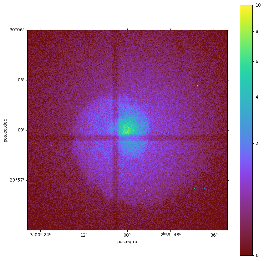
Now we can take a quick look at the image:

soxs.plot_image(
    "img.fits", stretch="sqrt", cmap="arbre", vmin=0.0, vmax=10.0, width=0.2
)

(<Figure size 1000x1000 with 2 Axes>, <WCSAxes: >)