pyXSIM Example

To show how to make a set of photons from a 3D dataset using pyXSIM and yt for reading into SOXS, we’ll look at is that of thermal emission from a galaxy cluster. In this case, the gas in the core of the cluster is “sloshing” in the center, producing spiral-shaped cold fronts. The dataset we want to use for this example is available for download from the yt Project at this link.

First, import our necessary modules:

import yt
import pyxsim
import soxs

Next, we load the dataset with yt (this dataset does not have species fields, so we specify that the gas is fully ionized in this case so that the emission measure field can be computed correctly):

ds = yt.load(
    "GasSloshing/sloshing_nomag2_hdf5_plt_cnt_0150", default_species_fields="ionized"
)

yt : [INFO     ] 2024-04-15 22:18:50,449 Parameters: current_time              = 1.1835090993823291e+17

yt : [INFO     ] 2024-04-15 22:18:50,449 Parameters: domain_dimensions         = [16 16 16]

yt : [INFO     ] 2024-04-15 22:18:50,450 Parameters: domain_left_edge          = [-3.70272e+24 -3.70272e+24 -3.70272e+24]

yt : [INFO     ] 2024-04-15 22:18:50,450 Parameters: domain_right_edge         = [3.70272e+24 3.70272e+24 3.70272e+24]

yt : [INFO     ] 2024-04-15 22:18:50,450 Parameters: cosmological_simulation   = 0

Let’s use yt to take a slice of density and temperature through the center of the dataset so we can see what we’re looking at:

slc = yt.SlicePlot(
    ds, "z", [("gas", "density"), ("gas", "temperature")], width=(1.0, "Mpc")
)
slc.show()

yt : [INFO     ] 2024-04-15 22:18:50,963 xlim = -1542838790481162406985728.000000 1542838790481162406985728.000000

yt : [INFO     ] 2024-04-15 22:18:50,963 ylim = -1542838790481162406985728.000000 1542838790481162406985728.000000

yt : [INFO     ] 2024-04-15 22:18:50,965 xlim = -1542838790481162406985728.000000 1542838790481162406985728.000000

yt : [INFO     ] 2024-04-15 22:18:50,965 ylim = -1542838790481162406985728.000000 1542838790481162406985728.000000

yt : [INFO     ] 2024-04-15 22:18:50,970 Making a fixed resolution buffer of (('gas', 'density')) 800 by 800

yt : [INFO     ] 2024-04-15 22:18:51,310 Making a fixed resolution buffer of (('gas', 'temperature')) 800 by 800

Ok, sloshing gas as advertised. Next, we’ll create a sphere object to serve as a source for the photons. Place it at the center of the domain with "c", and use a radius of 500 kpc:

sp = ds.sphere("c", (0.5, "Mpc"))

Now, we need to set up the emission model for our source. We said we were going to look at the thermal emission from the hot plasma, so we’ll do that here by using ThermalSourceModel. The first four arguments are the name of the underlying spectral model, the maximum and minimum energies, and the number of bins in the spectrum. We’ve chosen these numbers so that the spectrum has an energy resolution of about 1 eV. Setting thermal_broad=True turns on thermal broadening. This simulation does not include metallicity, so we’ll do something simple and say that it uses the above spectral model and the metallicity is a constant \(Z = 0.3~Z_\odot\):

source_model = pyxsim.CIESourceModel(
    "apec", 0.5, 9.0, 9000, thermal_broad=True, Zmet=0.3
)

pyxsim : [INFO     ] 2024-04-15 22:18:52,056 kT_min = 0.025 keV

pyxsim : [INFO     ] 2024-04-15 22:18:52,057 kT_max = 64 keV

We’re almost ready to go to generate the photons from this source, but first we should decide what our redshift, collecting area, and exposure time should be. Let’s pick big numbers, because remember the point of this first step is to create a Monte-Carlo sample from which to draw smaller sub-samples for mock observations. Note these are all (value, unit) tuples:

exp_time = (300.0, "ks")  # exposure time
area = (3.0, "m**2")  # collecting area
redshift = 0.2

So, that’s everything–let’s create the photons!

n_photons, n_cells = pyxsim.make_photons(
    "my_photons", sp, redshift, area, exp_time, source_model
)

pyxsim : [INFO     ] 2024-04-15 22:18:52,069 Cosmology: h = 0.71, omega_matter = 0.27, omega_lambda = 0.73

pyxsim : [INFO     ] 2024-04-15 22:18:52,070 Using emission measure field '('gas', 'emission_measure')'.

pyxsim : [INFO     ] 2024-04-15 22:18:52,070 Using temperature field '('gas', 'temperature')'.

pyxsim : [INFO     ] 2024-04-15 22:27:13,051 Finished generating photons.

pyxsim : [INFO     ] 2024-04-15 22:27:13,054 Number of photons generated: 21413397

pyxsim : [INFO     ] 2024-04-15 22:27:13,055 Number of cells with photons: 4053626

Ok, that was easy. Now we have a photon list that we can use to create events, using the project_photons() function. To be realistic, we’re going to want to assume foreground Galactic absorption, using the “TBabs” absorption model and assuming a foreground absorption column of \(N_H = 4 \times 10^{20}~{\rm cm}^{-2}\). Here we’ll just do a simple projection along the z-axis, reducing the exposure time, and centering the photons at RA, Dec = (30, 45) degrees:

n_events = pyxsim.project_photons(
    "my_photons", "my_events", "z", (30.0, 45.0), absorb_model="tbabs", nH=0.04
)

pyxsim : [INFO     ] 2024-04-15 22:27:13,075 Foreground galactic absorption: using the tbabs model and nH = 0.04.

pyxsim : [INFO     ] 2024-04-15 22:27:21,380 Detected 19246123 events.

We can then use this event list that we wrote as an input to the instrument simulator in SOXS. We’ll use a smaller exposure time (100 ks instead of 500 ks), and observe it with the Lynx calorimeter:

soxs.instrument_simulator(
    "my_events.h5",
    "evt.fits",
    (100.0, "ks"),
    "lynx_lxm",
    [30.0, 45.0],
    overwrite=True,
)

soxs : [INFO     ] 2024-04-15 22:27:21,392 Making observation of source in evt.fits.

soxs : [INFO     ] 2024-04-15 22:27:22,156 Detecting events from source my_events.

soxs : [INFO     ] 2024-04-15 22:27:22,158 Applying energy-dependent effective area from xrs_mucal_3x10_3.0eV.arf.

soxs : [INFO     ] 2024-04-15 22:27:24,308 Pixeling events.

soxs : [INFO     ] 2024-04-15 22:27:24,717 Scattering events with a image-based PSF.

soxs : [INFO     ] 2024-04-15 22:27:25,011 2629988 events were detected from the source.

soxs : [INFO     ] 2024-04-15 22:27:25,095 Scattering energies with RMF xrs_mucal_3.0eV.rmf.

soxs : [INFO     ] 2024-04-15 22:27:31,195 Adding background events.

soxs : [INFO     ] 2024-04-15 22:27:31,289 Adding in point-source background.

soxs : [INFO     ] 2024-04-15 22:27:31,509 Detecting events from source ptsrc_bkgnd.

soxs : [INFO     ] 2024-04-15 22:27:31,510 Applying energy-dependent effective area from xrs_mucal_3x10_3.0eV.arf.

soxs : [INFO     ] 2024-04-15 22:27:31,519 Pixeling events.

soxs : [INFO     ] 2024-04-15 22:27:31,524 Scattering events with a image-based PSF.

soxs : [INFO     ] 2024-04-15 22:27:31,529 32312 events were detected from the source.

soxs : [INFO     ] 2024-04-15 22:27:31,530 Scattering energies with RMF xrs_mucal_3.0eV.rmf.

soxs : [INFO     ] 2024-04-15 22:27:32,096 Generated 32312 photons from the point-source background.

soxs : [INFO     ] 2024-04-15 22:27:32,096 Adding in astrophysical foreground.

soxs : [INFO     ] 2024-04-15 22:27:49,388 Adding in instrumental background.

soxs : [INFO     ] 2024-04-15 22:27:49,452 Making 72027 events from the galactic foreground.

soxs : [INFO     ] 2024-04-15 22:27:49,452 Making 0 events from the instrumental background.

soxs : [INFO     ] 2024-04-15 22:27:49,506 Writing events to file evt.fits.

soxs : [INFO     ] 2024-04-15 22:27:49,993 Observation complete.

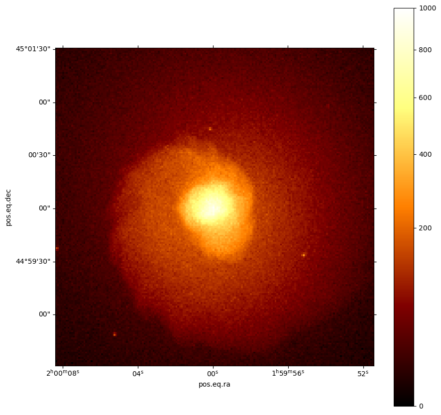
We can use the write_image() function in SOXS to bin the events into an image and write them to a file, restricting the energies between 0.5 and 2.0 keV:

soxs.write_image("evt.fits", "img.fits", emin=0.5, emax=2.0, overwrite=True)

We can show the resulting image:

fig, ax = soxs.plot_image(
    "img.fits", stretch="sqrt", cmap="afmhot", vmax=1000.0, width=0.05
)

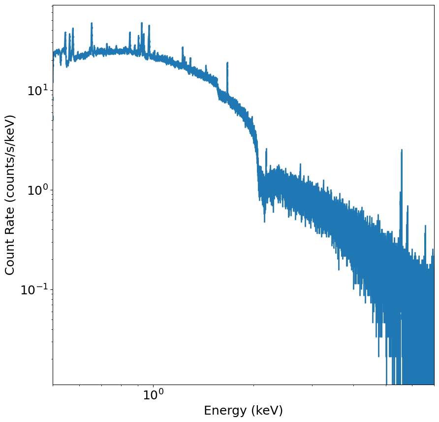
We can also bin the events into a spectrum using write_spectrum() and write the spectrum to disk:

soxs.write_spectrum("evt.fits", "evt.pha", overwrite=True)

and plot the spectrum using plot_spectrum():

fig, ax = soxs.plot_spectrum("evt.pha", xmin=0.5, xmax=7.0)

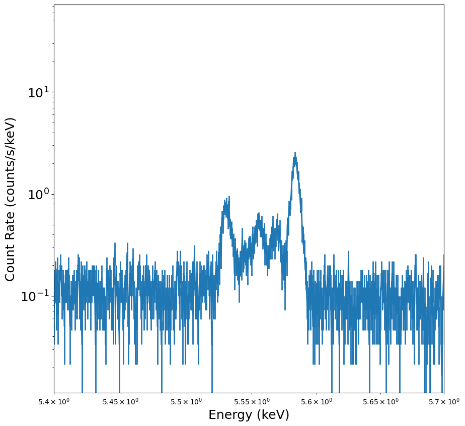
Let’s zoom into the region of the spectrum around the iron line to look at the detailed structure afforded by the resolution of the calorimeter:

ax.set_xlim(5.4, 5.7)
fig