Two Clusters

Using the SOXS Python interface, this example shows how to generate photons from two thermal spectra and two \(\beta\)-model spatial distributions, as an approximation of two galaxy clusters.

import matplotlib

matplotlib.rc("font", size=18)
import soxs

Generate Spectral Models

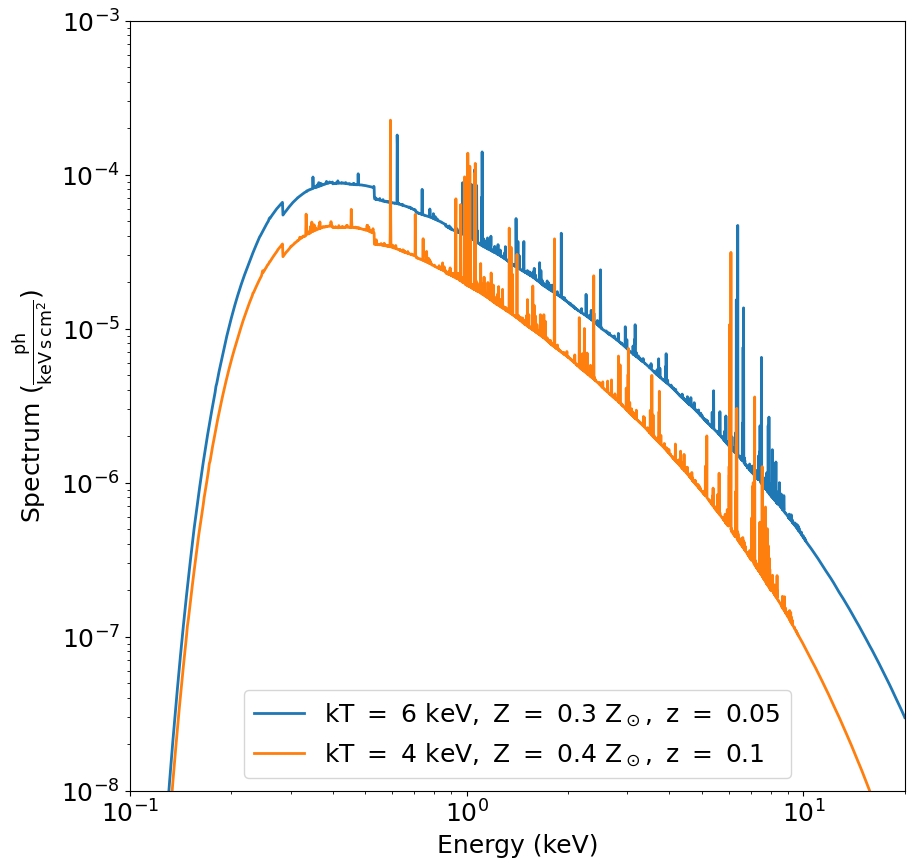
We want to generate thermal spectra, so we first create a spectral generator using the ApecGenerator class:

emin = 0.05  # keV
emax = 20.0  # keV
nbins = 20000
agen = soxs.ApecGenerator(emin, emax, nbins)

Next, we’ll generate the two thermal spectra. We’ll set the APEC norm for each to 1, and renormalize them later:

kT1 = 6.0
abund1 = 0.3
redshift1 = 0.05
norm1 = 1.0
spec1 = agen.get_spectrum(kT1, abund1, redshift1, norm1)

kT2 = 4.0
abund2 = 0.4
redshift2 = 0.1
norm2 = 1.0
spec2 = agen.get_spectrum(kT2, abund2, redshift2, norm2)

Now, re-normalize the spectra using energy fluxes between 0.5-2.0 keV:

flux1 = 1.0e-13  # erg/s/cm**2
flux2 = 5.0e-14  # erg/s/cm**2
emin = 0.5  # keV
emax = 2.0  # keV
spec1.rescale_flux(flux1, emin=0.5, emax=2.0, flux_type="energy")
spec2.rescale_flux(flux2, emin=0.5, emax=2.0, flux_type="energy")

We’ll also apply foreground galactic absorption to each spectrum:

n_H = 0.04  # 10^20 atoms/cm^2
spec1.apply_foreground_absorption(n_H)
spec2.apply_foreground_absorption(n_H)

spec1 and spec2 are Spectrum objects. Let’s have a look at the spectra:

fig, ax = spec1.plot(
    xmin=0.1,
    xmax=20.0,
    ymin=1.0e-8,
    ymax=1.0e-3,
    label="$\mathrm{kT\ =\ 6\ keV,\ Z\ =\ 0.3\ Z_\odot,\ z\ =\ 0.05}$",
)
spec2.plot(
    label="$\mathrm{kT\ =\ 4\ keV,\ Z\ =\ 0.4\ Z_\odot,\ z\ =\ 0.1}$", fig=fig, ax=ax
)
ax.legend()

<>:6: SyntaxWarning: invalid escape sequence '\m'
<>:9: SyntaxWarning: invalid escape sequence '\m'
<>:6: SyntaxWarning: invalid escape sequence '\m'
<>:9: SyntaxWarning: invalid escape sequence '\m'
/var/folders/6n/s0lf9frd7zq68c7dhlr090y4c91lh9/T/ipykernel_60544/1595130315.py:6: SyntaxWarning: invalid escape sequence '\m'
  label="$\mathrm{kT\ =\ 6\ keV,\ Z\ =\ 0.3\ Z_\odot,\ z\ =\ 0.05}$",
/var/folders/6n/s0lf9frd7zq68c7dhlr090y4c91lh9/T/ipykernel_60544/1595130315.py:9: SyntaxWarning: invalid escape sequence '\m'
  label="$\mathrm{kT\ =\ 4\ keV,\ Z\ =\ 0.4\ Z_\odot,\ z\ =\ 0.1}$", fig=fig, ax=ax

<matplotlib.legend.Legend at 0x146fcd490>

Generate Spatial Models

Now what we want to do is associate spatial distributions with these spectra. Each cluster will be represented using a \(\beta\)-model. For that, we use the BetaModel class. For fun, we’ll give the second BetaModel an ellipticity and tilt it by 45 degrees (a bit extreme, but it demonstrates the functionality nicely):

# Parameters for the clusters
r_c1 = 30.0  # in arcsec
r_c2 = 20.0  # in arcsec
beta1 = 2.0 / 3.0
beta2 = 1.0

# Center of the field of view
ra0 = 30.0  # degrees
dec0 = 45.0  # degrees

# Space the clusters roughly a few arcminutes apart on the sky.
# They're at different redshifts, so one is behind the other.
dx = 3.0 / 60.0  # degrees
ra1 = ra0 - 0.5 * dx
dec1 = dec0 - 0.5 * dx
ra2 = ra0 + 0.5 * dx
dec2 = dec0 + 0.5 * dx

# Now actually create the models
pos1 = soxs.BetaModel(ra1, dec1, r_c1, beta1, ellipticity=0.5, theta=45.0)
pos2 = soxs.BetaModel(ra2, dec2, r_c2, beta2)

Create SIMPUT files

Now, what we want to do is generate energies and positions from these models. We want to create a large sample that we’ll draw from when we run the instrument simulator, so we choose a large exposure time and a large collecting area (should be bigger than the maximum of the ARF). To do this, we use the from_models() method of the SimputPhotonList class to make instances of the latter:

t_exp = (500.0, "ks")
area = (3.0, "m**2")
cluster_phlist1 = soxs.SimputPhotonList.from_models(
    "cluster1", spec1, pos1, t_exp, area
)
cluster_phlist2 = soxs.SimputPhotonList.from_models(
    "cluster2", spec2, pos2, t_exp, area
)

soxs : [INFO     ] 2024-04-15 22:17:47,976 Creating 1537615 energies from this spectrum.

soxs : [INFO     ] 2024-04-15 22:17:48,108 Finished creating energies.

soxs : [INFO     ] 2024-04-15 22:17:48,431 Creating 729213 energies from this spectrum.

soxs : [INFO     ] 2024-04-15 22:17:48,489 Finished creating energies.

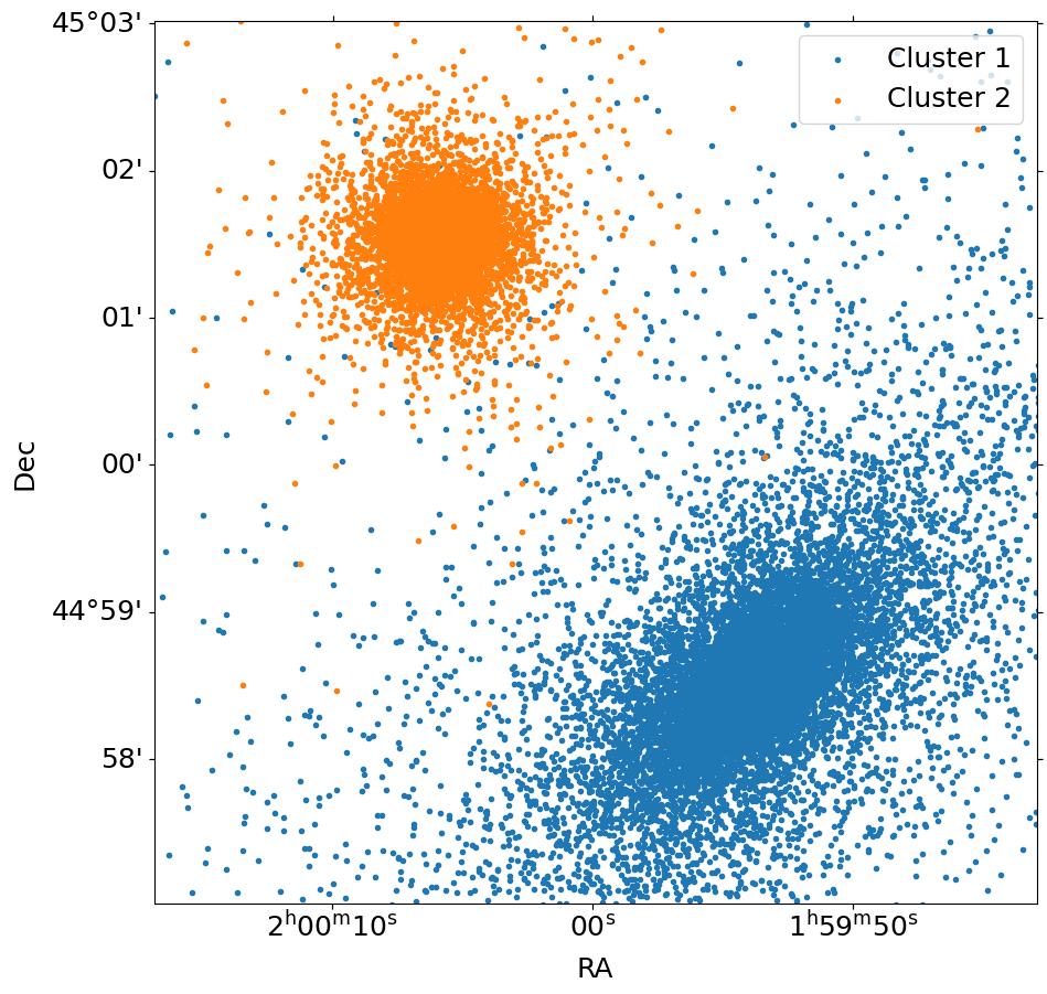
We can quickly show the positions using the plot() method of the SimputPhotonList instances. For simplicity, we’ll only show every 100th event using the stride argument, and restrict ourselves to a roughly \(20'\times~20'\) field of view.

fig, ax = cluster_phlist1.plot(
    [30.0, 45.0], 6.0, marker=".", stride=100, label="Cluster 1"
)
cluster_phlist2.plot(
    [30.0, 45.0], 6.0, marker=".", stride=100, fig=fig, ax=ax, label="Cluster 2"
)
ax.legend()

<matplotlib.legend.Legend at 0x164c83380>

Now that we have the positions and the energies of the photons in the SimputPhotonLists, we can write them to a SIMPUT catalog, using the SimputCatalog class. Each cluster will have its own photon list, but be part of the same SIMPUT catalog:

# Create the SIMPUT catalog "sim_cat" from the photon lists "cluster1" and "cluster2"
sim_cat = soxs.SimputCatalog.from_source(
    "clusters_simput.fits", cluster_phlist1, overwrite=True
)
sim_cat.append(cluster_phlist2)

soxs : [INFO     ] 2024-04-15 22:17:49,364 Appending source 'cluster1' to clusters_simput.fits.

soxs : [INFO     ] 2024-04-15 22:17:49,482 Appending source 'cluster2' to clusters_simput.fits.

Simulate an Observation

Finally, we can use the instrument simulator to simulate the two clusters by ingesting the SIMPUT file, setting an output file "evt.fits", setting an exposure time of 50 ks (less than the one we used to generate the source), the "lynx_hdxi" instrument, and the pointing direction of (RA, Dec) = (30.,45.) degrees.

soxs.instrument_simulator(
    "clusters_simput.fits",
    "evt.fits",
    (50.0, "ks"),
    "lynx_hdxi",
    [30.0, 45.0],
    overwrite=True,
)

soxs : [INFO     ] 2024-04-15 22:17:49,511 Making observation of source in evt.fits.

soxs : [INFO     ] 2024-04-15 22:17:49,636 Detecting events from source cluster1.

soxs : [INFO     ] 2024-04-15 22:17:49,636 Applying energy-dependent effective area from xrs_hdxi_3x10.arf.

soxs : [INFO     ] 2024-04-15 22:17:49,673 Pixeling events.

soxs : [INFO     ] 2024-04-15 22:17:49,683 Scattering events with a image-based PSF.

soxs : [INFO     ] 2024-04-15 22:17:49,696 74511 events were detected from the source.

soxs : [INFO     ] 2024-04-15 22:17:49,712 Detecting events from source cluster2.

soxs : [INFO     ] 2024-04-15 22:17:49,713 Applying energy-dependent effective area from xrs_hdxi_3x10.arf.

soxs : [INFO     ] 2024-04-15 22:17:49,730 Pixeling events.

soxs : [INFO     ] 2024-04-15 22:17:49,735 Scattering events with a image-based PSF.

soxs : [INFO     ] 2024-04-15 22:17:49,740 38855 events were detected from the source.

soxs : [INFO     ] 2024-04-15 22:17:49,742 Scattering energies with RMF xrs_hdxi.rmf.

soxs : [INFO     ] 2024-04-15 22:17:50,355 Adding background events.

soxs : [INFO     ] 2024-04-15 22:17:50,422 Adding in point-source background.

soxs : [INFO     ] 2024-04-15 22:17:52,377 Detecting events from source ptsrc_bkgnd.

soxs : [INFO     ] 2024-04-15 22:17:52,378 Applying energy-dependent effective area from xrs_hdxi_3x10.arf.

soxs : [INFO     ] 2024-04-15 22:17:52,549 Pixeling events.

soxs : [INFO     ] 2024-04-15 22:17:52,675 Scattering events with a image-based PSF.

soxs : [INFO     ] 2024-04-15 22:17:52,776 811580 events were detected from the source.

soxs : [INFO     ] 2024-04-15 22:17:52,803 Scattering energies with RMF xrs_hdxi.rmf.

soxs : [INFO     ] 2024-04-15 22:17:54,186 Generated 811580 photons from the point-source background.

soxs : [INFO     ] 2024-04-15 22:17:54,187 Adding in astrophysical foreground.

soxs : [INFO     ] 2024-04-15 22:18:05,528 Adding in instrumental background.

soxs : [INFO     ] 2024-04-15 22:18:05,801 Making 8545347 events from the galactic foreground.

soxs : [INFO     ] 2024-04-15 22:18:05,801 Making 101963 events from the instrumental background.

soxs : [INFO     ] 2024-04-15 22:18:06,406 Writing events to file evt.fits.

soxs : [INFO     ] 2024-04-15 22:18:08,126 Observation complete.

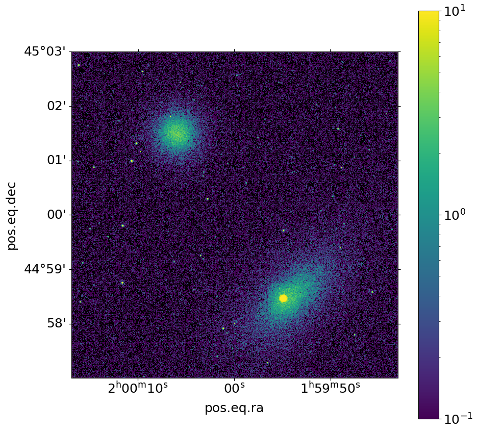
We can use the write_image() function in SOXS to bin the events into an image and write them to a file, restricting the energies between 0.5 and 2.0 keV:

soxs.write_image("evt.fits", "img.fits", emin=0.5, emax=2.0, overwrite=True)

Now we show the resulting image:

fig, ax = soxs.plot_image(
    "img.fits", stretch="log", cmap="viridis", vmin=0.1, vmax=10.0, width=0.1
)

Alternative Way to Generate the SIMPUT Catalog

In the above example, we generated the SIMPUT catalog for the observation of the two clusters using SimputPhotonLists, which in previous versions was the only option available in SOXS. It is also possible to use two SimputSpectrum objects, which is another type of SIMPUT source that consists of a spectrum and (optionally) an image. The image is used by SOXS to serve as a model to generate photon positions on the sky. If no image is included, then the source is simply a point source.

In this case of course, the clusters are two extended sources, so we can use the from_models method in a similar way as we did above, but in this case we have to supply the width and the resolution (nx) of the image that we want to associate with the spectrum:

width = 10.0  # arcmin by default
nx = 1024  # resolution of image
cluster_spec1 = soxs.SimputSpectrum.from_models("cluster1", spec1, pos1, width, nx)
cluster_spec2 = soxs.SimputSpectrum.from_models("cluster2", spec2, pos2, width, nx)

Then we create the SIMPUT catalog in essentially the same way as before:

# Create the SIMPUT catalog "sim_cat" from the spectra "cluster1" and "cluster2" in the same way
sim_cat2 = soxs.SimputCatalog.from_source(
    "clusters2_simput.fits", cluster_spec1, overwrite=True
)
sim_cat2.append(cluster_spec2)

soxs : [INFO     ] 2024-04-15 22:18:16,122 Appending source 'cluster1' to clusters2_simput.fits.

soxs : [INFO     ] 2024-04-15 22:18:16,168 Appending source 'cluster2' to clusters2_simput.fits.

Run the instrument_simulator:

soxs.instrument_simulator(
    "clusters2_simput.fits",
    "evt2.fits",
    (50.0, "ks"),
    "lynx_hdxi",
    [30.0, 45.0],
    overwrite=True,
)

soxs : [INFO     ] 2024-04-15 22:18:16,180 Making observation of source in evt2.fits.

soxs : [INFO     ] 2024-04-15 22:18:16,290 Detecting events from source cluster1.

soxs : [INFO     ] 2024-04-15 22:18:16,290 Applying energy-dependent effective area from xrs_hdxi_3x10.arf.

soxs : [INFO     ] 2024-04-15 22:18:16,332 Pixeling events.

soxs : [INFO     ] 2024-04-15 22:18:16,341 Scattering events with a image-based PSF.

soxs : [INFO     ] 2024-04-15 22:18:16,349 75571 events were detected from the source.

soxs : [INFO     ] 2024-04-15 22:18:16,356 Detecting events from source cluster2.

soxs : [INFO     ] 2024-04-15 22:18:16,356 Applying energy-dependent effective area from xrs_hdxi_3x10.arf.

soxs : [INFO     ] 2024-04-15 22:18:16,384 Pixeling events.

soxs : [INFO     ] 2024-04-15 22:18:16,388 Scattering events with a image-based PSF.

soxs : [INFO     ] 2024-04-15 22:18:16,393 38421 events were detected from the source.

soxs : [INFO     ] 2024-04-15 22:18:16,394 Scattering energies with RMF xrs_hdxi.rmf.

soxs : [INFO     ] 2024-04-15 22:18:16,988 Adding background events.

soxs : [INFO     ] 2024-04-15 22:18:17,057 Adding in point-source background.

soxs : [INFO     ] 2024-04-15 22:18:19,248 Detecting events from source ptsrc_bkgnd.

soxs : [INFO     ] 2024-04-15 22:18:19,248 Applying energy-dependent effective area from xrs_hdxi_3x10.arf.

soxs : [INFO     ] 2024-04-15 22:18:19,479 Pixeling events.

soxs : [INFO     ] 2024-04-15 22:18:19,643 Scattering events with a image-based PSF.

soxs : [INFO     ] 2024-04-15 22:18:19,769 1121036 events were detected from the source.

soxs : [INFO     ] 2024-04-15 22:18:19,804 Scattering energies with RMF xrs_hdxi.rmf.

soxs : [INFO     ] 2024-04-15 22:18:21,472 Generated 1121036 photons from the point-source background.

soxs : [INFO     ] 2024-04-15 22:18:21,473 Adding in astrophysical foreground.

soxs : [INFO     ] 2024-04-15 22:18:32,766 Adding in instrumental background.

soxs : [INFO     ] 2024-04-15 22:18:33,047 Making 8541647 events from the galactic foreground.

soxs : [INFO     ] 2024-04-15 22:18:33,047 Making 101639 events from the instrumental background.

soxs : [INFO     ] 2024-04-15 22:18:33,627 Writing events to file evt2.fits.

soxs : [INFO     ] 2024-04-15 22:18:34,729 Observation complete.

and make an image:

soxs.write_image("evt2.fits", "img2.fits", emin=0.5, emax=2.0, overwrite=True)
fig, ax = soxs.plot_image(
    "img2.fits", stretch="log", cmap="viridis", vmin=0.1, vmax=10.0, width=0.1
)

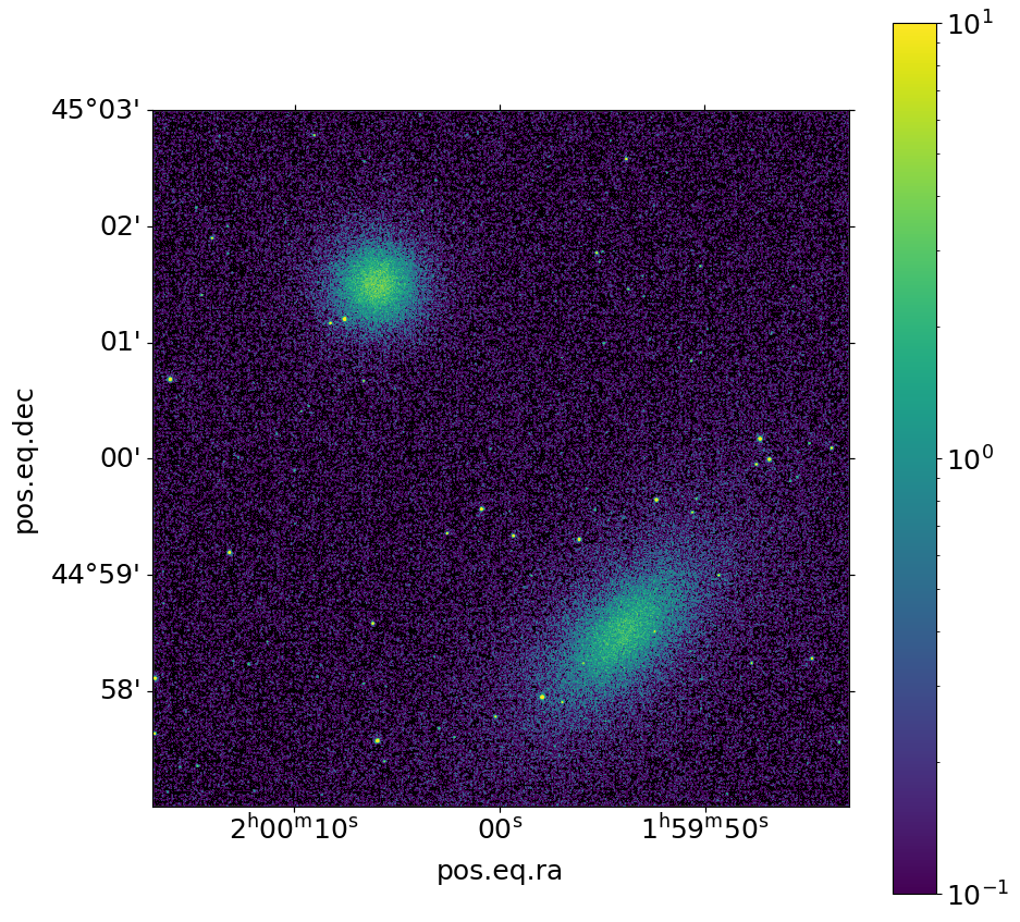
We used the same models, so the resulting images are the same except that different random numbers were used.