Creating and Using Spectra
SOXS provides a way to create common types of spectra that can then be
used in your scripts to create mock observations via the
Spectrum object.
Spectrum Binning
The energy binning of spectral tables can be either linear or log–that is, either the difference between the minimum and maximum energies of each bin is constant across the spectrum (linear) or that the difference between the logarithm of the minimum and maximum energies of each bin is constant across the spectrum (log).
For most of the spectrum creation methods outlined below, there will be the following keyword arguments to control the binning of spectral tables:
emin: The minimum energy of the spectral table in keV.emax: The maximum energy of the spectral table in keV.nbins: The number of bins in the spectrum.binscale: An optional argument which takes either"linear"or"log". The default is always"linear".
Creating Spectrum Objects
A Spectrum object is simply defined by a table
of energies and photon fluxes. There are several ways to create a
Spectrum, depending on your use case.
Creating a Constant Spectrum
A simple constant spectrum can be created using the
from_constant() method. This takes as input the
value of the flux const_flux, which is in units of
emin, emax, nbins, and binscale are used to control the binning.
const_flux = 1.0e-7
emin = 0.1
emax = 10.0
nbins = 20000
spec = Spectrum.from_constant(const_flux, emin, emax, nbins, binscale="linear")
Creating a Power-Law Spectrum
A simple power-law spectrum can be created using the
from_powerlaw() method. This takes as input
a spectral index photon_index, a redshift redshift, and a normalization
of the source norm at 1 keV in the source frame, in units of
where photon_index (note the sign convention). The parameters
emin, emax, nbins, and binscale are used to control the binning.
You can set up a power-law spectrum like this:
alpha = 1.2
zobs = 0.05
norm = 1.0e-7
emin = 0.1
emax = 10.0
nbins = 20000
spec = Spectrum.from_powerlaw(alpha, zobs, norm, emin, emax, nbins, binscale="log")
Generating a Spectrum from XSPEC or pyXspec
If you have XSPEC installed on
your machine, you can use it with SOXS to create any spectral model that XSPEC
supports. You can do this in three ways. The first is by passing in a model
string and a list of parameters to the
from_xspec_model() method:
model_string = "phabs*(mekal+powerlaw)" # A somewhat complicated model
params = [0.02, 6.0, 1.0, 0.3, 0.03, 1, 0.01, 1.2, 1.0e-3]
emin = 0.1
emax = 5.0
nbins = 20000
spec = Spectrum.from_xspec_model(model_string, params, emin, emax, nbins)
Note that the parameters must be in the same order that they would be if you
were entering them in XSPEC. The parameters emin, emax, nbins,
and binscale are used to control the binning.
The second way involves passing an XSPEC script file to the
from_xspec_script() method which defines an XSPEC
model. For example, a script that creates a model spectrum from a sum of two
APEC models may look like this:
statistic chi
method leven 10 0.01
abund angr
xsect bcmc
cosmo 70 0 0.73
xset delta 0.01
systematic 0
model  apec    +   apec
            0.2       0.01      0.008      0.008         64         64
              1     -0.001          0          0          5          5
              0      -0.01     -0.999     -0.999         10         10
    6.82251e-07       0.01          0          0      1e+24      1e+24
          0.099       0.01      0.008      0.008         64         64
              1     -0.001          0          0          5          5
              0      -0.01     -0.999     -0.999         10         10
    1.12328e-06       0.01          0          0      1e+24      1e+24
If it is contained within the file "two_apec.xcm", it can be used to
create a Spectrum like this:
emin = 0.1
emax = 5.0
nbins = 20000
spec = Spectrum.from_xspec_script("two_apec.xcm", emin, emax, nbins,
                                  binscale="log")
The parameters emin, emax, nbins, and binscale are used to
control the binning.
For either from_xspec_model() or
from_xspec_script(), you can pass a dictionary xspec_settings which
will apply a number of XSPEC settings before generating the spectral models. For example, you can
set the APECROOT and the APECTHERMAL variables in this way:
xspec_settings = {
    "APECROOT": "/path/to/apec",
    "APECTHERMAL": "",
}

spec = Spectrum.from_xspec_model(model_string, params, emin, emax, nbins,
                                 binscale="log", xspec_settings=xspec_settings)
Note that for settings that do not require values, one simply sets "" as the value in the
dictionary.
The third way is to use pyXspec
to generate a spectrum. This requires that pyXspec is installed as part of your HEASoft installation
and is installed into the same Python environment as SOXS. If so, you can create an xspec.Model
object in the usual way, and then pass it to the from_pyxspec_model()
method:
import soxs
import xspec

# Set energy binning
xspec.AllData.dummyrsp(0.2, 2.0, 6000, "lin")

# Create a model
m = xspec.Model("phabs*(mekal+powerlaw)")

# Change some parameters
m.phabs.nH = 0.02
m.mekal.kT = 6.0
m.mekal.Abundanc = 0.3

# Get the spectrum
spec = soxs.Spectrum.from_pyxspec_model(m)
Note
Generating spectra from XSPEC or pyXspec requires that the HEADAS environment
variable is defined within your shell before running the Python script or notebook,
as it would be if you were using XSPEC/pyXspec to fit spectra. For example, for the
zsh shell there should be a line like
export HEADAS=${HOME}/heasoft-6.29/x86_64-apple-darwin21.1.0/ in your .zshrc
file.
Math with Spectrum Objects
Two Spectrum objects can be co-added, provided that
they have the same energy binning:
spec1 = Spectrum.from_powerlaw(1.1, 0.05, 1.0e-9, 0.1, 10.0, 10000)
spec2 = agen.get_spectrum(6.0, 0.3, 0.05, 1.0e-3)

total_spectrum = spec1 + spec2
If they do not, an error will be thrown.
Or they can be subtracted:
diff_spectrum = spec1-spec2
You can also multiply a spectrum by a constant float number or divide it by one:
spec3 = 6.0*spec2
spec4 = spec1/4.4
Attributes of Spectrum Objects
The Spectrum object has a number of unitful attributes
which may be helpful for the end-user, which are shown here.
from soxs import Spectrum

spec = Spectrum.from_powerlaw(1.1, 0.05, 1.0e-9, 0.1, 10.0, 10000)

print(spec.ebins) # the energy bin edges
print()
print(spec.emid) # the energy bin centers
print()
print(spec.de) # the energy bin widths
print()
print(spec.flux) # the photon flux per energy bin
print()
print(spec.energy_flux) # the energy flux per energy bin
print()
[ 0.1      0.10099  0.10198 ...  9.99802  9.99901 10.     ] keV

[0.100495 0.101485 0.102475 ... 9.997525 9.998515 9.999505] keV

[0.00099 0.00099 0.00099 ... 0.00099 0.00099 0.00099] keV

[1.18667795e-08 1.17395035e-08 1.16148084e-08 ... 7.53026088e-11
 7.52944072e-11 7.52862073e-11] ph / (keV s cm2)

[1.91067895e-18 1.90880682e-18 1.90695468e-18 ... 1.20618220e-18
 1.20617026e-18 1.20615831e-18] erg / (keV s cm2)
There are also a number of per-wavelength or per-frequency versions of the above:
print(spec.wvbins) # the wavelength bin edges
print()
print(spec.wvmid) # the wavelength bin centers
print()
print(spec.dwv) # the wavelength bin widths
print()
print(spec.flux_per_wavelength) # the photon flux per wavelength bin
print()
print(spec.energy_flux_per_wavelength) # the energy flux per wavelength bin
print()
[123.98419843 122.76878744 121.57697434 ...   1.24008752   1.23996474
 1.23984198] Angstrom

[123.37649294 122.17288089 120.99252642 ...   1.24014892   1.24002613
 1.23990336] Angstrom

[1.21541100e+00 1.19181310e+00 1.16889584e+00 ... 1.22805138e-04
 1.22780820e-04 1.22756509e-04] Angstrom
print(spec.fbins) # the frequency bin edges
print()
print(spec.fmid) # the frequency bin centers
print()
print(spec.df) # the frequency bin widths
print()
print(spec.flux_per_frequency) # the photon flux per frequency bin
print()
print(spec.energy_flux_per_frequency) # the energy flux per frequency bin
print()
[2.41798924e+16 2.44192734e+16 2.46586543e+16 ... 2.41751048e+18
 2.41774986e+18 2.41798924e+18] Hz

[2.42995829e+16 2.45389638e+16 2.47783448e+16 ... 2.41739079e+18
 2.41763017e+18 2.41786955e+18] Hz

[2.39380935e+14 2.39380935e+14 2.39380935e+14 ... 2.39380935e+14
 2.39380935e+14 2.39380935e+14] Hz

[4.90770565e-26 4.85506854e-26 4.80349881e-26 ... 3.11426567e-28
 3.11392648e-28 3.11358735e-28] ph / (Hz s cm2)

[7.90193322e-36 7.89419073e-36 7.88653087e-36 ... 4.98836876e-36
 4.98831936e-36 4.98826997e-36] erg / (Hz s cm2)
Getting the Values and Total Flux or Luminosity of a Spectrum Within a Specific Energy Band
A new Spectrum object can be created from a restricted
energy band of an existing one by calling the new_spec_from_band()
method:
emin = 0.5
emax = 7.0
subspec = spec.new_spec_from_band(emin, emax)
The get_flux_in_band() method can be used
to quickly report on the total flux within a specific energy band within
the observer frame:
emin = 0.5
emax = 7.0
print(spec.get_flux_in_band(emin, emax))
which returns a tuple of the photon flux and the energy flux, showing:
(<Quantity 2.2215588675210208e-07 ph / (cm2 s)>,
 <Quantity 7.8742710307246895e-16 erg / (cm2 s)>)
The get_lum_in_band() method can also be used
to quickly report on the total luminosity and count rate within a specific
energy band, where in this case the band in question is the rest frame of
the source. For this reason, either a redshift must be supplied, or for a
local source a distance must be given.
emin = 0.5
emax = 7.0
print(spec.get_lum_in_band(emin, emax, redshift=0.05))
which returns a tuple of the photon count rate and the luminosity, showing:
(<Quantity 1.35081761e+48 ph / s>, <Quantity 4.78819407e+39 erg / s>)
You can change the cosmology as well by supplying a Cosmology
object to cosmology (otherwise the Planck 2018 cosmology is assumed):
from astropy.cosmology import WMAP9
emin = 0.5
emax = 7.0
print(spec.get_lum_in_band(emin, emax, redshift=0.05, cosmology=WMAP9))
See the AstroPy cosmology documentation for more details.
You can supply a distance for a local source (redshift assumed zero) like this:
emin = 0.5
emax = 7.0
print(spec.get_lum_in_band(emin, emax, dist=(8.0, "kpc")))
Finally, Spectrum objects are “callable”, and if one
supplies a single energy or array of energies, the values of the spectrum
at these energies will be returned. AstroPy Quantity
objects are detected and handled appropriately.
print(spec(3.0)) # energy assumed to be in keV
<Quantity 2.830468922349541e-10 ph / (cm2 keV s)>
from astropy.units import Quantity
# AstroPy quantity, units will be converted to keV internally
e = Quantity([1.6e-9, 3.2e-9, 8.0e-9], "erg")
print(spec(e)) # energy assumed to be in keV
<Quantity [ 9.47745587e-10, 4.42138950e-10, 1.61370731e-10] ph / (cm2 keV s)>
Rescaling the Normalization of a Spectrum
You can rescale the normalization of the entire spectrum using the
rescale_flux() method. This can be
helpful when you want to set the normalization of the spectrum by the
total flux within a certain energy band instead.
spec.rescale_flux(1.0e-9, emin=0.5, emax=7.0, flux_type="photons"):
emin and emax can be used to set the band that the flux corresponds to.
If they are not set, they are assumed to be the bounds of the spectrum. The flux
type can be "photons" (the default) or "energy". In the former case, the
units of the new flux must be
Applying Galactic Foreground Absorption to a Spectrum
The apply_foreground_absorption() method
can be used to apply foreground absorption using the "wabs" or
"tbabs" models. It takes one required parameter, the hydrogen
column along the line of sight, in units of "model"
parameter (default is "wabs"):
spec = Spectrum.from_powerlaw(1.1, 0.05, 1.0e-9, 0.1, 10.0, 10000)
n_H = 0.02
spec.apply_foreground_absorption(n_H, model="tbabs")
The flux in the energy bins will be reduced according to the absorption at a
given energy. Optionally, to model absorption intrinsic to a source or
from a source intermediate between us and the source, one can supply an
optional redshift argument (default 0.0):
spec = Spectrum.from_powerlaw(1.1, 0.05, 1.0e-9, 0.1,
                              10.0, 10000)
n_H = 0.02
spec.apply_foreground_absorption(n_H, model="tbabs", redshift=0.05)
Finally, the abundance table for the "tbabs" absorption model can be
specified (the default is "angr"):
spec = Spectrum.from_powerlaw(1.1, 0.05, 1.0e-9, 0.1,
                              10.0, 10000)
n_H = 0.02
spec.apply_foreground_absorption(n_H, model="tbabs", redshift=0.05,
                                 abund_table="wilm")
See Changing the Solar Abundance Table for options for different abundance tables.
The current version for the "tbabs" model is 2.3.2.
Adding Emission Lines to a Spectrum
The add_emission_line() method adds a single Gaussian
emission line to an existing Spectrum object. The
line energy, line width, and amplitude of the line (the line strength or
integral under the curve) must be specified. The formula for the emission
line is:
where
spec = Spectrum.from_powerlaw(1.1, 0.05, 1.0e-9, 0.1,
                              10.0, 10000)
line_center = (6.0, "keV") # "E_0" above
line_width = (30.0, "eV") # "FWHM" above
line_amp = (1.0e-7, "photon/s/cm**2") # "A" above
spec.add_emission_line(line_center, line_width, line_amp)
The line width may also be specified in units of velocity, if that is more convenient:
spec = Spectrum.from_powerlaw(1.1, 0.05, 1.0e-9, 0.1,
                              10.0, 10000)
line_center = (6.0, "keV")
line_width = (200.0, "km/s")
line_amp = (1.0e-7, "photon/s/cm**2")
spec.add_emission_line(line_center, line_width, line_amp)
Currently, this functionality only supports emission lines with a Gaussian shape.
Adding Absorption Lines to a Spectrum
The add_absorption_line() method adds a single Gaussian
absorption line to an existing Spectrum object. The
line energy, line width, and equivalent width of the line must be specified.
The formula for the absorption line is given in terms of the optical depth
where
and the strength of the absorption
where
spec = Spectrum.from_powerlaw(1.1, 0.05, 1.0e-9, 0.1,
                              10.0, 10000)
line_center = (1.0, "keV") # "E_0" above
line_width = (30.0, "eV") # "FWHM" above
equiv_width = 2 # defaults to units of milli-Angstroms
spec.add_absorption_line(line_center, line_width, equiv_width)
The line width may also be specified in units of velocity, if that is more convenient:
spec = Spectrum.from_powerlaw(1.1, 0.05, 1.0e-9, 0.1,
                              10.0, 10000)
line_center = (1.0, "keV")
line_width = (500.0, "km/s")
equiv_width = (3.0e-3, "Angstrom")
spec.add_absorption_line(line_center, line_width, equiv_width)
Currently, this functionality only supports absorption lines with a Gaussian shape.
Generating Photon Energies From a Spectrum
Given a Spectrum, a set of photon energies can be
drawn from it using the generate_energies()
method. This will most often be used to generate discrete samples for mock
observations. For this method, an exposure time and a constant
(energy-independent) effective area must be supplied to convert the spectrum’s
flux to a number of photons. These values need not be realistic–in fact, they
both should be larger than the values for the mock observation that you want to
simulate, to create a statistically robust sample to draw photons from when we
actually pass them to the instrument simulator.
An example using a Spectrum created from a file:
spec = Spectrum.from_file("my_spec.dat")
t_exp = (100., "ks") # exposure time
area = (3.0, "m**2") # constant effective area
energies = spec.generate_energies(t_exp, area)
The energies object generate_energies() returns
is an augmented NumPy array which also carries the unit information and the total
flux of energies:
print(energies.unit)
print(energies.flux)
Unit("keV")
<Quantity 1.1256362913845828e-15 erg / (cm2 s)>
Normally, generate_energies() will not need to be
called by the end-user but will be used “under the hood” in the generation of
a PhotonList as part of a SimputCatalog.
See SIMPUT for more information.
Count Rate Spectra
The CountRateSpectrum class is basically the same thing as a
the Spectrum class, except that it is in units of
One important note about CountRateSpectrum objects is that you
can also call generate_energies() on them, except
that unlike Spectrum objects it is not necessary to specify an area,
but only an exposure time, to generate energies:
# here "spec" is a CountRateSpectrum object
t_exp = (100., "ks") # exposure time
energies = spec.generate_energies(t_exp)
“Convolved” Spectra
One may want to examine a spectrum after it has been convolved with a particular
effective area curve. One can generate such a
ConvolvedSpectrum using the
convolve() method, feeding it a
Spectrum object and an ARF:
from soxs import ConvolvedSpectrum
# Assuming one created an ApecGenerator agen...
spec2 = agen.get_spectrum(6.0, 0.3, 0.05, 1.0e-3)
cspec = ConvolvedSpectrum.convolve(spec2, "xrs_hdxi_3x10.arf")
The spectrum in this object has units of
Spectrum’s methods on it. For example, to determine the
count and energy rate within a particular band:
cspec.get_flux_in_band(0.5, 7.0)
(<Quantity 6.802363401824924 ph / s>,
 <Quantity 1.2428592072628134e-08 erg / s>)
Or to generate an array of energies:
t_exp = (500.0, "ks")
e = cspec.generate_energies(t_exp)
If one has already loaded a AuxiliaryResponseFile,
then one can also generate a ConvolvedSpectrum by simply
multiplying the ARF by a Spectrum object:
from soxs import AuxiliaryResponseFile
arf = AuxiliaryResponseFile("xrs_hdxi_3x10.arf")
# Assuming one created an ApecGenerator agen...
spec2 = agen.get_spectrum(6.0, 0.3, 0.05, 1.0e-3)
cspec = spec2*arf
To “deconvolve” a ConvolvedSpectrum object and return
a Spectrum object, simply call
deconvolve():
spec_new = cspec.deconvolve()
Including an RMF in the Convolution
It is also possible to include an RMF in the convolution process. This will take
the spectrum which has been convolved with the ARF and further convolve it with
with the response matrix in the RMF. This will produce a spectrum with features
that have been broadened by the energy resolution of the instrument. This may be
useful for comparing model Spectrum objects to mock observations
by forward-modeling them through the instrument responses. To do this, simply pass
the name of the RMF file to convolve():
from soxs import ConvolvedSpectrum
# Assuming one created an ApecGenerator agen...
spec2 = agen.get_spectrum(6.0, 0.3, 0.05, 1.0e-3)
cspec = ConvolvedSpectrum.convolve(spec2, "xrs_hdxi_3x10.arf",
                                   rmf="xrs_hdxi.rmf")
Note
If one uses an RMF to convolve, the methods
generate_energies() and
deconvolve() are not available.
Plotting Spectra
All Spectrum objects and their associated subclasses have
a plot() method which can be used to make a
Matplotlib plot. The plot()
method has no required arguments, but has a number of optional arguments for plot
customization. This method returns a tuple of the Figure and
the Axes objects to allow for further customization. This
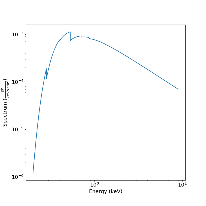
example shows how to make a simple plot of an absorbed power-law spectrum:
spec = soxs.Spectrum.from_powerlaw(1.2, 0.02, 1.0e-3, 0.2, 9.0, 100000)
spec.apply_foreground_absorption(0.1)
fig, ax = spec.plot()
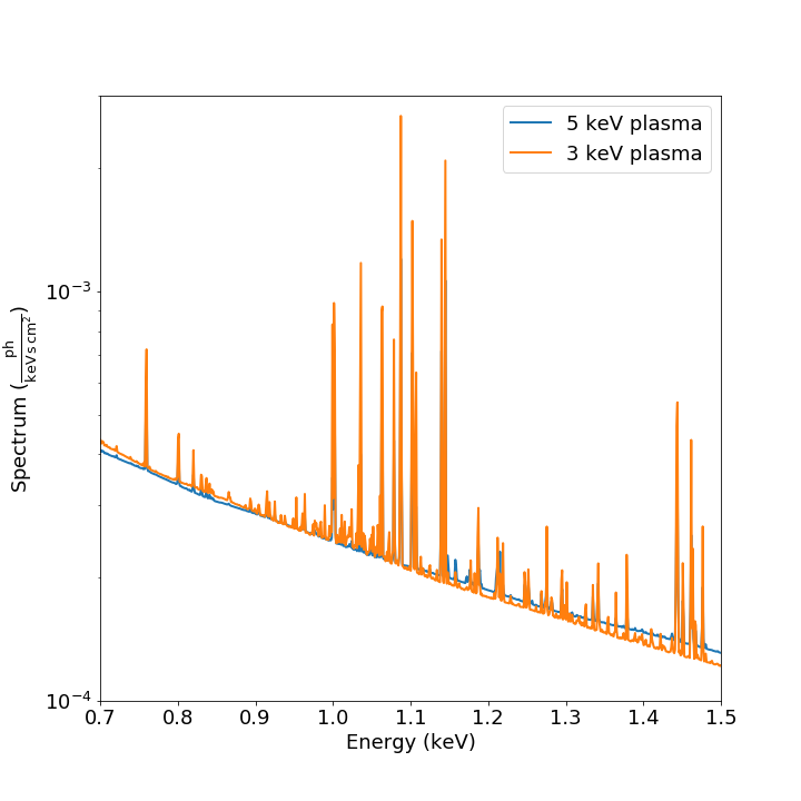
Here’s another example of creating a plot of two thermal spectra with labels, zooming in on a section of it, and setting the energy scale to linear:
agen = soxs.ApecGenerator(0.1, 10.0, 10000)
spec1 = agen.get_spectrum(5.0, 0.3, 0.02, 1.0e-3)
spec2 = agen.get_spectrum(3.0, 0.3, 0.02, 1.0e-3)
fig, ax = spec1.plot(xmin=0.7, xmax=1.5, ymin=1.0e-4, ymax=3.0e-3,
                     xscale='linear', label="5 keV plasma")
spec2.plot(fig=fig, ax=ax, label="3 keV plasma")
For other customizations, consult the plot() API.
Writing a Spectrum to Disk
Spectrum objects can be written to disk in three formats:
an ASCII text file in the ECSV format, a FITS file, or an HDF5 file. To write a
spectrum to an ASCII ECSV file, use the write_ascii_file()
method:
agen = soxs.ApecGenerator(0.1, 10.0, 10000)
spec1 = agen.get_spectrum(5.0, 0.3, 0.02, 1.0e-3)
spec1.write_ascii_file("my_spec.ecsv", overwrite=True)
To write a spectrum to an HDF5 file, use write_hdf5_file():
agen = soxs.ApecGenerator(0.1, 10.0, 10000)
spec1 = agen.get_spectrum(5.0, 0.3, 0.02, 1.0e-3)
spec1.write_hdf5_file("my_spec.h5", overwrite=True)
To write a spectrum to a FITS file, use write_fits_file():
agen = soxs.ApecGenerator(0.1, 10.0, 10000)
spec1 = agen.get_spectrum(5.0, 0.3, 0.02, 1.0e-3)
spec1.write_fits_file("my_spec.fits", overwrite=True)
In each case, the minimum and maximum energies for each bin in the table, the
flux in each bin (as well as its units), and the bin scaling (linear or log)
is written to the file. If writing a ConvolvedSpectrum
object, the name of the ARF which was used to do the convolution is also stored.
Reading a Spectrum from Disk
Spectrum objects written using any of the writing methods
detailed above (ASCII ECSV, HDF5, or FITS) can be the spectrum can be read back
in again in, using from_file():
from soxs import Spectrum
my_spec = Spectrum.from_file("my_spec.ecsv")
Special I/O for Convolved Spectra
ConvolvedSpectrum objects can be written directly to
PI/PHA files using the same standard format that is used for real spectra,
with the to_pha_file() method:
from soxs import ConvolvedSpectrum
# Assuming one created an ApecGenerator agen...
spec2 = agen.get_spectrum(6.0, 0.3, 0.05, 1.0e-3)
cspec = ConvolvedSpectrum.convolve(spec2, "xrs_hdxi_3x10.arf")
cspec.to_pha_file("my_spec.pi", overwrite=True)
Conversely, PI/PHA files produced can be read in as ConvolvedSpectrum
objects:
import soxs
cspec = soxs.ConvolvedSpectrum.from_pha_file("my_spec.pi")