The AstroStat Slog

RMF. It is a wørd to strike terror even into the hearts of the intrepid. It refers to the spread in the measured energy of an incoming photon, and even astronomers often stumble over what it is and what it contains. It essentially sets down the measurement error for registering the energy of a photon in the given instrument.

Thankfully, its usage is robustly built into analysis software such as Sherpa or XSPEC and most people don’t have to deal with the nitty gritty on a daily basis. But given the profusion of statistical software being written for astronomers, it is perhaps useful to go over what it means. Continue reading ‘Redistribution’ »

Like spherical cows, true blackbodies do not exist. Not because “black objects are dark, duh”, as I’ve heard many people mistakenly say — black here simply refers to the property of the object where no wavelength is preferentially absorbed or emitted, and all the energy input to it is converted into radiation. There are many famous astrophysical cases which are very good approximations to perfect blackbodies — the 2.73K microwave background radiation left over from the early Universe, for instance. Even the Sun is a good example. So it is often used to model the emission from various objects. Continue reading ‘Blackbody Radiation [Eqn]’ »

I still remember my first class as a new grad student. As a cocky Physics graduate, I was quite sure I knew plenty of astronomy. Astro 301, class 1, and it took all of 20 minutes of talk about stellar magnitudes to put that notion to permanent rest. So, for the sake of our stats colleagues, here’s a brief primer on one of the basic building blocks of astronomy. Continue reading ‘Magnitude [Eqn]’ »

Differential Emission Measures (DEMs) are a summary of the temperature structure of the outer atmospheres (aka coronae) of stars, and are usually derived from a select subset of line fluxes. They are notoriously difficult to estimate. Very few algorithms even bother to calculate error envelopes on them. They are also subject to numerous systematic uncertainties which can play havoc with proper interpretation. But they are nevertheless extremely useful since they allow changes in coronal structures to be easily discerned, and observations with one instrument can be used to derive these DEMs and these can then be used to predict what is observable with some other instrument. Continue reading ‘Differential Emission Measure [Eqn]’ »

I grew up in an environment that glamourized mathematical equations. Equations adorned a text like jewelry, set there to dazzle, and often to outshine the text that they were to illuminate. Needless to say, anything I wrote was dense, opaque, and didn’t communicate what it set out to. It was not until I saw a Reference Frame essay by David Mermin on how to write equations (1989, Physics Today, 42, p9) that I realized that equations should be treated as part of the text. You should be able to read them. David Mermin set out 3 rules for writing out equations, which I’ve tried to follow diligently (if not always successfully) since then. Continue reading ‘I Like Eq’ »

As mentioned before, background subtraction plays a big role in astrophysical analyses. For a variety of reasons, it is not a good idea to subtract out background counts from source counts, especially in the low-counts Poisson regime. What Bayesians recommend instead is to set up a model for the intensity of the source and the background and to infer these intensities given the data. Continue reading ‘Background Subtraction, the Sequel [Eqn]’ »

I have noticed that our statistician collaborators are often confused by our units. (Not a surprise; I, too, am constantly confused by our units.) One of the biggest culprits is the unit of energy, [keV], Continue reading ‘keV vs keV [Eqn]’ »

With the LHC coming on line anon, it is appropriate to highlight the Banff Challenge, which was designed as a way to figure out how to place bounds on the mass of the Higgs boson. The equations that were to be solved are quite general, and are in fact the first attempt that I know of where calibration data are directly and explicitly included in the analysis. Continue reading ‘The Banff Challenge [Eqn]’ »

The Χ² distribution plays an incredibly important role in astronomical data analysis, but it is pretty much a black box to most astronomers. How many people know, for instance, that its form is exactly the same as the γ distribution? A Χ² distribution with ν degrees of freedom is

p(z|ν) = (1/Γ(ν/2)) (1/2)^ν/2 z^ν/2-1 e^-z/2 ≡ γ(z;ν/2,1/2) , where z=Χ².

Continue reading ‘chi-square distribution [Eqn]’ »

The Kaplan-Meier (K-M) estimator is the non-parametric maximum likelihood estimator of the survival probability of items in a sample. “Survival” here is a historical holdover because this method was first developed to estimate patient survival chances in medicine, but in general it can be thought of as a form of cumulative probability. It is of great importance in astronomy because so much of our data are limited and this estimator provides an excellent way to estimate the fraction of objects that may be below (or above) certain flux levels. The application of K-M to astronomy was explored in depth in the mid-80′s by Jurgen Schmitt (1985, ApJ, 293, 178), Feigelson & Nelson (1985, ApJ 293, 192), and Isobe, Feigelson, & Nelson (1986, ApJ 306, 490). [See also Hyunsook's primer.] It has been coded up and is available for use as part of the ASURV package. Continue reading ‘Kaplan-Meier Estimator (Equation of the Week)’ »

Astrophysics, especially high-energy astrophysics, is all about counting photons. And this, it is said, naturally leads to all our data being generated by a Poisson process. True enough, but most astronomers don’t know exactly how it works out, so this derivation is for them. Continue reading ‘Poisson Likelihood [Equation of the Week]’ »

For a discipline that relies so heavily on images, it is rather surprising how little use astronomy makes of the vast body of work on image analysis carried out by mathematicians and computer scientists. Mathematical morphology, for example, can be extremely useful in enhancing, recognizing, and extracting useful information from densely packed astronomical
images.

The building blocks of mathematical morphology are two operators, Erode[I|Y] and Dilate[I|Y], Continue reading ‘Open and Shut [Equation of the Week]’ »

From Protassov et al. (2002, ApJ, 571, 545), here is a formal expression for the Likelihood Ratio Test Statistic,

T_LRT = -2 ln R(D,Θ₀,Θ)

R(D,Θ₀,Θ) = [ sup_θεΘ0 p(D|Θ₀) ] / [ sup_θεΘ p(D|Θ) ]

where D are an independent data sample, Θ are model parameters {θ_i, i=1,..M,M+1,..N}, and Θ₀ form a subset of the model where θ_i = θ_i⁰, i=1..M are held fixed at their nominal values. That is, Θ represents the full model and Θ₀ represents the simpler model, which is a subset of Θ. R(D,Θ₀,Θ) is the ratio of the maximal (technically, supremal) likelihoods of the simpler model to that of the full model.
Continue reading ‘Likelihood Ratio Test Statistic [Equation of the Week]’ »

High-resolution astronomical spectroscopy has invariably been carried out with gratings. Even with the advent of the new calorimeter detectors, which can measure the energy of incoming photons to an accuracy of as low as 1 eV, gratings are still the preferred setups for hi-res work below energies of 1 keV or so. But how do they work? Where are the sources of uncertainty, statistical or systematic?
Continue reading ‘Grating Dispersion [Equation of the Week]’ »

X-ray telescopes generally work by reflecting photons at grazing incidence. As you can imagine, even small imperfections in the mirror polishing will show up as huge roadbumps to the incoming photons, and the higher their energy, the easier it is for them to scatter off their prescribed path. So X-ray telescopes tend to have sharp peaks and fat tails compared to the much more well-behaved normal-incidence telescopes, whose PSFs (Point Spread Functions) can be better approximated as Gaussians.

X-ray telescopes usually also have gratings that can be inserted into the light path, so that photons of different energies get dispersed by different angles, and whose actual energies can then be inferred accurately by measuring how far away on the detector they ended up. The accuracy of the inference is usually limited by the width of the PSF. Thus, a major contributor to the LRF (Line Response Function) is the aforementioned scattering.

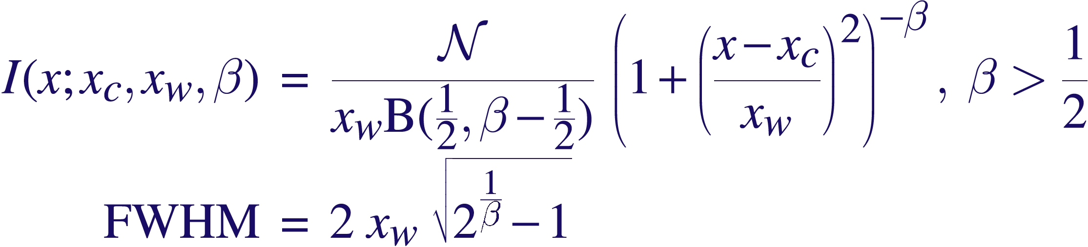
A correct accounting of the spread of photons of course requires a full-fledged response matrix (RMF), but as it turns out, the line profiles can be fairly well approximated with Beta profiles, which are simply Lorentzians modified by taking them to the power β –

where B(1/2,β-1/2) is the Beta function, and N is a normalization constant defined such that integrating the Beta profile over the real line gives the area under the curve as N. The parameter β controls the sharpness of the function — the higher the β, the peakier it gets, and the more of it that gets pushed into the wings. Chandra LRFs are usually well-modeled with β~2.5, and XMM/RGS appears to require Lorentzians, β~1.

The form of the Lorentzian may also be familiar to people as the Cauchy Distribution, which you get for example when the ratio is taken of two quantities distributed as zero-centered Gaussians. Note that the mean and variance are undefined for that distribution.