Simulation for XMM spectra (AO-4)
Last modified:
February 26, 2007
This thread uses
PINTofALE
to generate simulated XMM EPIC-PN, EPIC-MOS, and RGS spectra
of a coronal source normalized to a ROSAT/PSPC count rate.
The XMM ARF, RMF and RSP files used here can be obtained from the
PROPOSAL & PLANNING TOOLS page.
- Initialize variables
- Define a DEM
- Rescale DEM to match ROSAT count rate
- Construct spectra
- Simulate and plot
- Comparison with PIMMS
All the steps described here are repeated in the .par file:
XMM_epic_rgs_ao4.par.
0. Initialize the settings
#	start IDL
idl

;	set up the PoA environment
;
.run initale

;NOTE:
;	if INITALE fails, run the script
;	@PoA_constructor
1. Initialize some variables
;	Because some variables will be used repeatedly in the course of this
;	thread, it might be useful to initialize them now. Nailing down these
;	variables now will also allow for something of a checklist for some
;	important quantities/files needed for the task at hand:

;	Local Environment We will set up the pathnames specific to
;	the local installation here

 !LDBDIR = '$CHIANTI'		; Atomic Line Database
		; choose from the predefined '$CHIANTI', '$SPEX', '$APED',
		; or specify the full path name to the line database

 pimmsdir='/soft/pimms/data'	; the full path name to the PIMMS database

;	Source We will characterize our model source by the following:

 !NH           = 3e20			 ; H column density [cm^-2]
 !EDENS        = 1.0e9   		 ; electron number density [cm^-3]
 !ABUND        = getabund('grevesse et al.') ; element abundances
					     ;(SEE: getabund())
 T_components  = [6.1, 6.8, 7.2]		; log(T[K]) components in EM
 EM_components = [6.1d11, 6.1d11, 7.1e11]	; Emission Measure [cm^-3]

;	Observation The observation can be described by:

 EXPTIME       =  50.			; nominal exposure time [ks]
 obs_rate      = 0.1                    ; ROSAT/PSPC count rate [ct/s]
					; (set to 0 or less to be ignored)

 pn_ARF        = 'pn-medium.arf'   	; EPIC-PN ARF filename or 'none'
 mos_ARF       = 'mos1-medium.arf' 	; EPIC-MOS ARF filename or 'none'
 rgs1_ARF      = 'none'			; RGS1 ARF filename or 'none'
 rgs2_ARF      = 'none'			; RGS2 ARF filename or 'none'
 pn_RMF        = 'pn.rmf'	     	; EPIC-PN RMF filename
 mos_RMF       = 'mos1.rmf'        	; EPIC-MOS RMF filename
 rgs1_RMF      = 'RGS1ORDER1.RSP'  	; RGS-1 RMF filename
 rgs2_RMF      = 'RGS2ORDER1.RSP'  	; RGS-2 RMF filename

;NOTE: the standard RGS response matrices include the
;effective area, and hence an ARF should not be specified for them.

;	Analysis Parameters
;       We may restrict the analysis to the wavelength ranges of interest.
;       Here we set the ROSAT/PSPC passband used to measure obs_rate,
;       the desired XMM output passband, and the wavelength grid
;       for the idealized model spectrum. The output spectra will be
;       defined on the default response energy grids restricted to
;       the ranges defined here.

 emin_rosat = 0.12	; minimum energy in ROSAT/PSPC passband [keV]
 emax_rosat = 2.48	; maximum energy in ROSAT/PSPC passband [keV]
 emin_xmm = 0.2         ; minimum energy in XMM passband [keV]
 emax_xmm = 8.0 	; maximum energy in XMM passband [keV]
 wmin_rosat = !fundae.kevang/emax_rosat ; convert to [Ang]
 wmax_rosat = !fundae.kevang/emin_rosat ; convert to [Ang]
 wmin_xmm = !fundae.kevang/emax_xmm ; convert to [Ang]
 wmax_xmm = !fundae.kevang/emin_xmm ; convert to [Ang]
 !WMIN = wmin_rosat < wmin_xmm ; minimum wavelength for model [Ang]
 !WMAX = wmax_rosat > wmax_xmm ; maximum wavelength for model [Ang]
 nwbin   =  10000L ; number of bins in model spectrum
2. Define a DEM
;	A Differential Emission Measure (DEM) is required to estimate the
;	amount of emission at various temperatures. Typically, a 2-temperature
;	model is used. Here we will use PINTofALE's mk_dem(), which constructs
;	a DEM array given a temperature grid and emission measure components.
;	We use as the temperature grid !LOGT. The emission measure components
;	are T_components and EM_components as defined above. We choose 'delta'
;	to treat the EM components as delta functions (see mk_dem() or the
;	Chandra/ACIS example for more options)

!DEM=mk_dem('delta', logT = !LOGT, pardem=T_components, indem=EM_components)
3. Rescale the DEM to match ROSAT count rate
;	We will assume that a ROSAT/PSPC count rate is available,
;	and that the simulation will match this rate.  We will assume
;	a count rate of 0.1 cts/s .  Data from other missions such
;	as ASCA, BeppoSAX, etc. can be dealt with in the same manner.

;	First find and read in the ROSAT/PSPC effective area.
;	You will need to know where your local PIMMS installation
;	is to do this.

rosat_pspc_open=get_pimms_file('ROSAT','PSPC','OPEN',pdir=pimmsdir)
rd_pimms_file, rosat_pspc_open, pspc_effar, pspc_wvlar, /wave

;	Make sure that the wavelengths are sorted in increasing order

ae=sort(pspc_wvlar) & pspc_wvlar=pspc_wvlar[ae] & pspc_effar=pspc_effar[ae]

;	The following is similar to the process described in the detailed
;	example thread (see Section 1 and Section 2)


A] Read in line cooling emissivities and calculate line intensities

;	Read line cooling emissivities of all possible lines in the
;	ROSAT/PSPC wavelength range from the atomic data base.

;	NOTE: To avoid multiple reads of the line emissivity database, we
;	shall read in the emissivities over the entire range of interest

lconf=rd_line(atom,n_e=!EDENS,$
	wrange=[MIN(pspc_wvlar)<!WMIN,MAX(pspc_wvlar)>!WMAX],$
	dbdir=!LDBDIR,verbose=!VERBOSE,wvl=LWVL,logT=LLOGT,Z=Z,$
	ion=ION,jon=JON,fstr=lstr)

;	The output of rd_line() will only include level population,
;	and not ion balances. We will use fold_ioneq() to fold ion balances.
;	NOTE: This step should not be performed if !LDBDIR is set to APED,
;	which already includes ion balances and abundances.

if strpos(strlowcase(!LDBDIR),'aped',0) lt 0 then lconf=$
	fold_ioneq(lconf,Z,JON,chidir=!CHIDIR,$
	logT=LLOGT,eqfile=!IONEQF,verbose=!VERBOSE)

;	And now calculate line intensities using lineflx().

v_ABUND = !ABUND
;	NOTE: If !LDBDIR is set to APED, Anders & Grevesse abundances
;	are already included in the emissivities.  In such cases, either
;	leave out the atomic numbers (Z) in the call to LINEFLX() below,
;	or redfine the abundance array to be relative to the APED values,
;	e.g.,
if strpos(strlowcase(!LDBDIR),'aped',0) ge 0 then $
	v_ABUND = !ABUND/getabund('anders & grevesse')

linint=lineflx(lconf,!LOGT,LWVL,Z,DEM=!DEM,abund=v_ABUND) ;[ph/s]


B] Read in continuum emissivities and calculate continuum intensities

;	We can read in continuum emissivities using rd_cont().
;	It is important to note that the output emissivities of rd_cont()
;	are in [1e-23 erg cm^3/s/Ang] and not [1e-23 erg cm^3/s] as with rd_line()

;	NOTE: To avoid multiple reads of the continuum emissivity database,
;	we shall read in the emissivities over the entire range of interest

cconf=rd_cont(!CEROOT,n_e=!EDENS,$
	wrange=[min(pspc_wvlar)<!WMIN,max(pspc_wvlar)>!WMAX],$
	dbdir=!CDBDIR,abund=!ABUND,verbose=!VERBOSE,$
	wvl=CWW,logT=ClogT)

;	The continuum intensities per angstrom can be calculated again using
;	lineflx(). Note that CWW contains the wavelength bin boundaries for
;	the emissivity array.

CWVL=0.5*(CWW[1:*]+CWW)
conint=lineflx(cconf,!LOGT,CWVL,DEM=!DEM)   ;[ph/s/Ang]

;	Now to get just continuum intensity, we must multiply by an array
;	containing the bin widths. If we define this array simply
;	with:  CDW=CWW[1:*]-CWW, we will get an ugly 'saw-toothed' figure.
;	(a side-effect of the way the data-base is constructed) To work
;	around this, we can use CWVL, the mid-bin values, and mid2bound(),
;	which gives intelligent bin-boundary values given mid-bin values:

CWB=mid2bound(CWVL) & CDW=CWB[1:*]-CWB
conint=conint*CDW	;[ph/s/Ang]*[Ang]


C] Correct for inter-stellar absorption

;	Derive ISM absorptions using ismtau()
ltau=ismtau(LWVL,NH=!NH,fH2=!fH2,He1=!He1,HeII=!HeII,$
	Fano=Fano,wam=wam,/bam,abund=!ABUND,verbose=!VERBOSE)
ctau=ismtau(CWVL,NH=!NH,fH2=!fH2,He1=!He1,HeII=!HeII,$
	Fano=Fano,wam=wam,/bam,abund=!ABUND,verbose=!VERBOSE)
ltrans=exp(-ltau) & ctrans=exp(-ctau)

;	Derive theoretical line fluxes
linflx = linint * ltrans	;[ph/s/cm^2]

;	Derive theoretical continuum fluxes
conflx = conint * ctrans	;[ph/s/cm^2]


D] Bin spectra and fold in effective area

;	make input theoretical spectrum grid
nwbin_pspc = n_elements(pspc_effar)
dwvl=float((max(pspc_wvlar)-min(pspc_wvlar))/nwbin_pspc)
wgrid=findgen(nwbin+1L)*dwvl+min(pspc_wvlar)

;	Rebin to form theoretical line spectrum using hastrogram()
linspc = hastogram(abs(LWVL),wgrid,wts=linflx)	;[ph/s/cm^2/bin]

;	Rebin to form theoretical continuum spectrum using rebinw()
conspc = rebinw(conflx,CWVL,wgrid,/perbin)	;[ph/s/cm^2/bin]

;	Derive predicted flux spectrum.
WVLS=0.5*(WGRID[1:*]+WGRID)
newEffAr=(interpol(pspc_effar,pspc_wvlar,WVLS) > 0) < (max(pspc_effar))
flxspc = (linspc + conspc) * newEffAr

;	Derive predicted counts spectrum.
flxspc=flxspc*EXPTIME*1e3		;[ct/bin]

;       Restrict the counts spectrum to the specified ACIS-I range
oo = where(wgrid ge wmin_rosat and wgrid le wmax_rosat)
flxspc = flxspc(oo)


;	Now get the total count rate and renormalize the DEM to the
;	observed rate of 0.1 ct/s.

pred_rate = total(flxspc/EXPTIME/1e3)       ;[ct/s]
print,''
if obs_rate gt 0 then $
	print,'Rescaling input DEM by a factor '+strtrim(obs_rate/pred_rate,2)
print,''
rescale_factor=1.0
if obs_rate gt 0 then rescale_factor = obs_rate/pred_rate
!DEM = !DEM * rescale_factor
linint = linint * rescale_factor
conint = conint * rescale_factor
linflx = linflx * rescale_factor
conflx = conflx * rescale_factor
4. Construct XMM Spectra
;       To construct the XMM spectra, we use the line and continuum
;	emissivities read in above (LCONF and CCONF), the line and
;	continuum intensities (LININT and CONINT) and fluxes (LINFLX
;	and CONFLX) computed above, and recompute the predicted fluxes
;	using XMM ARFs, and finally compute the observed spectra by
;	convolving with the RMFs.


A] Read in line cooling emissivities and calculate line intensities

	help,lconf,linint


B] Read in line cooling emissivities and calculate line intensities

	help,cconf,conint


C] Correct for inter-stellar absorption

	help,ltau,ltrans,linflx,ctau,ctrans,conflx


D] Bin spectra and fold in effective area

        EMAX = !fundae.kevang/!WMIN & EMIN = !fundae.kevang/!WMAX
        dnrg   = float((EMAX-EMIN)/nwbin)     ;  bin size
        egrid  = findgen(nwbin+1L)*dnrg+EMIN  ;  bin boundaries [keV]
        emid   = 0.5*(egrid[1:*]+egrid)       ;  mid-bin values [keV]
        wvls   = !fundae.kevang/emid          ;  [ang]

        linspc  = hastogram(!fundae.kevang/abs(LWVL),egrid,wts=linflx)  ; [ph/s/cm^2/bin]
        conspc  = rebinw(conflx,!fundae.kevang/CWB,egrid,/perbin)      ; [ph/s/cm^2/bin]

        ;Read in the effective areas using rdarf()

        if strlowcase(pn_ARF) eq 'none' then effar_pn=0*emid+1. else $
                effar_pn  = rdarf(pn_ARF,pn_ARF_str)
        if strlowcase(mos_ARF) eq 'none' then effar_mos=0*emid+1. else $
                effar_mos = rdarf(mos_ARF,mos_ARF_str)
        if strlowcase(rgs1_ARF) eq 'none' then effar_rgs1=0*emid+1. else $
                effar_rgs1 = rdarf(rgs1_ARF,rgs1_ARF_str)
        if strlowcase(rgs2_ARF) eq 'none' then effar_rgs2=0*emid+1. else $
                effar_rgs2 = rdarf(rgs2_ARF,rgs2_ARF_str)

        ;figure out the wavelength grid for effective areas

        if n_tags(pn_ARF_str) eq 0 then nrgar_pn=emid else $
          nrgar_pn = (0.5*(pn_ARF_str.ELO +pn_ARF_str.EHI))
        if n_tags(mos_ARF_str) eq 0 then nrgar_mos=emid else $
          nrgar_mos  = (0.5*(mos_ARF_str.ELO+mos_ARF_str.EHI))
        if n_tags(rgs1_ARF_str) eq 0 then nrgar_rgs1=emid else $
          nrgar_rgs1  = (0.5*(rgs1_ARF_str.ELO+rgs1_ARF_str.EHI))
        if n_tags(rgs2_ARF_str) eq 0 then nrgar_rgs2=emid else $
          nrgar_rgs2  = (0.5*(rgs2_ARF_str.ELO+rgs2_ARF_str.EHI))

        ;interpolate to put effective area on binned spectra grids

        new_effar_pn   = (interpol(effar_pn  ,nrgar_pn  ,EMID) > 0) < (max(effar_pn))
        new_effar_mos  = (interpol(effar_mos ,nrgar_mos ,EMID) > 0) < (max(effar_mos))
        new_effar_rgs1 = (interpol(effar_rgs1,nrgar_rgs1,EMID) > 0) < (max(effar_rgs1))
        new_effar_rgs2 = (interpol(effar_rgs2,nrgar_rgs2,EMID) > 0) < (max(effar_rgs2))

        ;[ct/s/bin] (if DEM is [cm-5]: [ct/s/cm2/bin])

        flxspc_pn   = (linspc + conspc) * new_effar_pn
        flxspc_mos  = (linspc + conspc) * new_effar_mos
        flxspc_rgs1 = (linspc + conspc) * new_effar_rgs1
        flxspc_rgs2 = (linspc + conspc) * new_effar_rgs2

        ;Derive predicted counts spectrum

        flxspc_pn    = flxspc_pn   *EXPTIME*1e3      ;[ct/bin]
        flxspc_mos   = flxspc_mos  *EXPTIME*1e3      ;[ct/bin]
        flxspc_rgs1  = flxspc_rgs1 *EXPTIME*1e3      ;[ct/bin]
        flxspc_rgs2  = flxspc_rgs2 *EXPTIME*1e3      ;[ct/bin]


E] Convolve with RMF using

;	read in RMFs
pn_RMF_str=rd_ogip_rmf(pn_RMF)
mos_RMF_str=rd_ogip_rmf(mos_RMF)
rgs1_RMF_str=rd_ogip_rmf(rgs1_RMF)
rgs2_RMF_str=rd_ogip_rmf(rgs2_RMF)

conv_rmf, egrid, flxspc_pn,   CHAN_pn,   CTSPC_pn,   pn_RMF_str
conv_rmf, egrid, flxspc_mos,  CHAN_mos,  CTSPC_mos,  mos_RMF_str
conv_rmf, egrid, flxspc_rgs1, CHAN_rgs1, CTSPC_rgs1, rgs1_RMF_str
conv_rmf, egrid, flxspc_rgs2, CHAN_rgs2, CTSPC_rgs2, rgs2_RMF_str


;	Get co-added RGS spectrum.

CHAN_rgs   = CHAN_rgs1                        ;[keV]
CTSPC_rgs  = CTSPC_rgs1 + CTSPC_rgs2          ;[ct/bin] valid grids same
flxspc_rgs = flxspc_rgs1+flx_spc_rgs2         ;[ct/bin] (if sperate ARF)

;       Restrict the spectra to the specified range
oo_rgs = where(CHAN_rgs gt emin_xmm and CHAN_rgs lt emax_xmm)
oo_mos = where(CHAN_mos gt emin_xmm and CHAN_mos lt emax_xmm)
oo_pn  = where(CHAN_pn  gt emin_xmm and CHAN_pn lt emax_xmm)

CTSPC_rgs1 = CTSPC_rgs1(oo_rgs) & CHAN_rgs1  = CHAN_rgs1(oo_rgs)
CTSPC_rgs2 = CTSPC_rgs2(oo_rgs) & CHAN_rgs2  = CHAN_rgs2(oo_rgs)
CTSPC_rgs  = CTSPC_rgs(oo_rgs)  & CHAN_rgs   = CHAN_rgs(oo_rgs)
CTSPC_mos  = CTSPC_mos(oo_mos)  & CHAN_mos   = CHAN_mos(oo_mos)
CTSPC_pn   = CTSPC_mos(oo_pn)   & CHAN_pn    = CHAN_pn(oo_pn)

;	Note that the output energy grid of the spectra will be by
;	default the energy grid defined by the RMF. The spectrum
;	however will only show lines and continuum between the
;	selected wavelength ranges.
5. Obtain Poisson deviates and plot
; The final step is a simulation of counts based on the spectrum
; predicted above
nbin_pn = n_elements(CTSPC_pn) & CTSIM_pn = intarr(nbin_pn)
nbin_mos = n_elements(CTSPC_mos) & CTSIM_mos = intarr(nbin_mos)
nbin_rgs = n_elements(CTSPC_rgs) & CTSIM_rgs = intarr(nbin_rgs)
for i=0L,nbin_pn-1L do if CTSPC_pn[i] gt 0 then $
CTSIM_pn[i] =randomu(seed,poisson=CTSPC_pn[i])
for i=0L,nbin_mos-1L do if CTSPC_mos[i] gt 0 then $
CTSIM_mos[i]=randomu(seed,poisson=CTSPC_mos[i])
for i=0L,nbin_rgs-1L do if CTSPC_rgs[i] gt 0 then $
CTSIM_rgs[i]=randomu(seed,poisson=CTSPC_rgs[i])
; The results of the calculations are plotted below
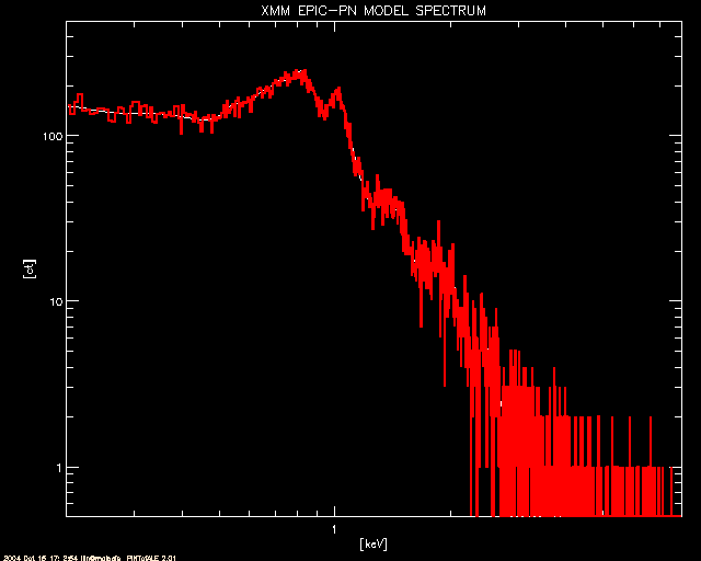
; The EPIC-pn model (in white) and simulated counts (in red)
window, 0
plot, CHAN_pn, CTSPC_pn, title='XMM EPIC-PN MODEL SPECTRUM',/xl,/yl,$
xtitle='[keV]', ytitle='[ct]', ystyle=1, xstyle=1, $
xrange=[emin_xmm,emax_xmm], yrange=[0.5,2*max(CTSPC_pn)] & stample
oplot, CHAN_pn, CTSIM_pn ,color = 2, psym=10, thick=2
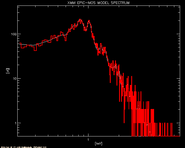
 ; The EPIC-mos model (in white) and simulated counts (in red)
window, 1
plot, CHAN_mos, CTSPC_mos, title='XMM EPIC-MOS MODEL SPECTRUM',/xl,/yl,$
xtitle='[keV]', ytitle='[ct]', ystyle=1, xstyle=1, $
xrange=[emin_xmm,emax_xmm], yrange=[0.5,2*max(CTSPC_mos)] & stample
oplot, CHAN_mos, CTSIM_mos, color = 2, psym=10, thick=2
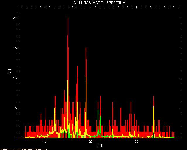
 ; The RGS model (in white) and simulated counts (in red). Also shown
; are the model counts from RGS1 (yellow) and RGS2 (green)
window, 2
plot, !fundae.kevang/CHAN_rgs, CTSIM_rgs, title='XMM RGS MODEL SPECTRUM',$
xtitle='['+!AA+']', ytitle='[ct]', ystyle=1, xstyle=1, /nodata,$
xrange=[!fundae.kevang/MAX(CHAN_rgs),!fundae.kevang/MIN(CHAN_rgs)],$
yrange=[0,1.1*max(CTSIM_rgs)]
oplot, !fundae.kevang/CHAN_rgs, CTSIM_rgs, color=2, psym=10, thick=2
oplot, !fundae.kevang/CHAN_rgs1, CTSPC_rgs1, color=3, psym=10, thick=2
oplot, !fundae.kevang/CHAN_rgs2, CTSPC_rgs2, color=4, psym=10, thick=2
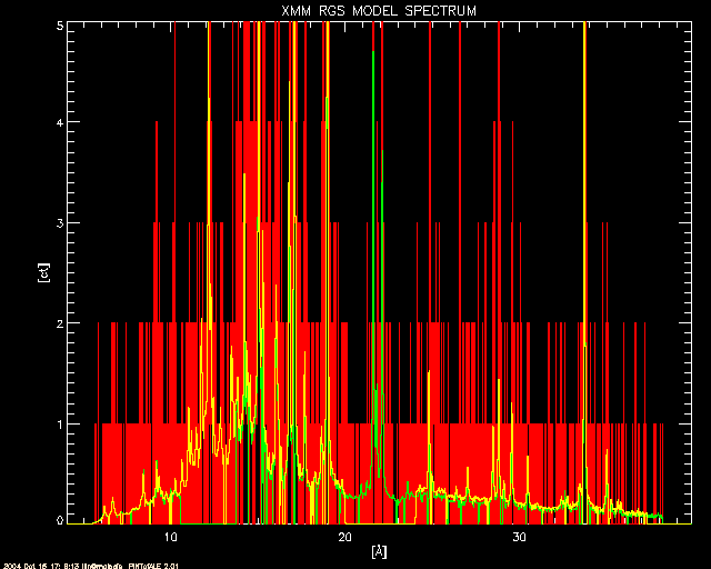
 ; As above, but zoomed in to show the low counts detail.
window, 3
plot, !fundae.kevang/CHAN_rgs, CTSIM_rgs, title='XMM RGS MODEL SPECTRUM',$
xtitle='['+!AA+']', ytitle='[ct]', ystyle=1, xstyle=1, /nodata,$
xrange=[!fundae.kevang/MAX(CHAN_rgs),!fundae.kevang/MIN(CHAN_rgs)],$
yrange=[0,5.*median(CTSPC_rgs)>5.]
oplot, !fundae.kevang/CHAN_rgs, CTSIM_rgs, color=2, psym=10
oplot, !fundae.kevang/CHAN_rgs1, CTSPC_rgs1, color=3, psym=10
oplot, !fundae.kevang/CHAN_rgs2, CTSPC_rgs2, color=4, psym=10
 ; We may summarize results as follows:
;
; Simulated counts spectra are in:
; CTSIM_pn(chan_pn),CTSIM_mos(CHAN_mos),CTSIM_rgs(CHAN_rgs) [ct/bin]
;
; Redistributed counts spectra are in:
; CTSPC_pn(chan_pn),CTSPC_mos(CHAN_mos),CTSPC_rgs(CHAN_rgs) [ct/bin]
;
; Predicted counts spectra are in:
; FLXSPC_pn(wvls),FLXSPC_mos(wvls), FLXSPC_rgs(wvls) [ct/bin]
;
; Note: Standard RGS response matrices include the effective area, so, unless
; a seperate rmf and effective area files are used, FLXSPC_rgs will
; NOT contain predicted counts spectra.
;
; Theoretical line fluxes are in:
; linspc(lwvl) [ph/s[/cm^2]]
;
; Theoretical continuum fluxes are in:
; conspc(cwvl) [ph/s[/cm^2]]
6. Comparison with PIMMS
;       Results using this thread  are roughly consistent with
;       PIMMS results. PIMMS returned the following XMM count rates
;       for a ROSAT/PSPC count rate of 0.1 cts/s and a Raymond-Smith
;       model of temperature 0.5437 keV:
;             XMM PN MED  :   7.792E-01 cts/s
;             XMM MOS MED :   1.958E-01 cts/s
;             XMM RGS1 O1 :   2.629E-02 cts/s
;             XMM RGS2 O1 :   3.627E-02 cts/s
;
;       Running this thread with  !ABUND = getabund('Allen'),
;       T_components = [6.8], and  obs_rate = 0.1 gives:
;             XMM PN MED  :  0.74  cts/s
;             XMM MOS MED :  0.19  cts/s
;             XMM RGS1 O1 :  0.027 cts/s
;             XMM RGS2 O1 :  0.035 cts/s
pintofale()head.cfa.harvard.edu (LL)
 ; The EPIC-mos model (in white) and simulated counts (in red)
window, 1
plot, CHAN_mos, CTSPC_mos, title='XMM EPIC-MOS MODEL SPECTRUM',/xl,/yl,$
xtitle='[keV]', ytitle='[ct]', ystyle=1, xstyle=1, $
xrange=[emin_xmm,emax_xmm], yrange=[0.5,2*max(CTSPC_mos)] & stample
oplot, CHAN_mos, CTSIM_mos, color = 2, psym=10, thick=2
 ; The RGS model (in white) and simulated counts (in red). Also shown
; are the model counts from RGS1 (yellow) and RGS2 (green)
window, 2
plot, !fundae.kevang/CHAN_rgs, CTSIM_rgs, title='XMM RGS MODEL SPECTRUM',$
xtitle='['+!AA+']', ytitle='[ct]', ystyle=1, xstyle=1, /nodata,$
xrange=[!fundae.kevang/MAX(CHAN_rgs),!fundae.kevang/MIN(CHAN_rgs)],$
yrange=[0,1.1*max(CTSIM_rgs)]
oplot, !fundae.kevang/CHAN_rgs, CTSIM_rgs, color=2, psym=10, thick=2
oplot, !fundae.kevang/CHAN_rgs1, CTSPC_rgs1, color=3, psym=10, thick=2
oplot, !fundae.kevang/CHAN_rgs2, CTSPC_rgs2, color=4, psym=10, thick=2
 ; As above, but zoomed in to show the low counts detail.
window, 3
plot, !fundae.kevang/CHAN_rgs, CTSIM_rgs, title='XMM RGS MODEL SPECTRUM',$
xtitle='['+!AA+']', ytitle='[ct]', ystyle=1, xstyle=1, /nodata,$
xrange=[!fundae.kevang/MAX(CHAN_rgs),!fundae.kevang/MIN(CHAN_rgs)],$
yrange=[0,5.*median(CTSPC_rgs)>5.]
oplot, !fundae.kevang/CHAN_rgs, CTSIM_rgs, color=2, psym=10
oplot, !fundae.kevang/CHAN_rgs1, CTSPC_rgs1, color=3, psym=10
oplot, !fundae.kevang/CHAN_rgs2, CTSPC_rgs2, color=4, psym=10
 ; We may summarize results as follows:
;
; Simulated counts spectra are in:
; CTSIM_pn(chan_pn),CTSIM_mos(CHAN_mos),CTSIM_rgs(CHAN_rgs) [ct/bin]
;
; Redistributed counts spectra are in:
; CTSPC_pn(chan_pn),CTSPC_mos(CHAN_mos),CTSPC_rgs(CHAN_rgs) [ct/bin]
;
; Predicted counts spectra are in:
; FLXSPC_pn(wvls),FLXSPC_mos(wvls), FLXSPC_rgs(wvls) [ct/bin]
;
; Note: Standard RGS response matrices include the effective area, so, unless
; a seperate rmf and effective area files are used, FLXSPC_rgs will
; NOT contain predicted counts spectra.
;
; Theoretical line fluxes are in:
; linspc(lwvl) [ph/s[/cm^2]]
;
; Theoretical continuum fluxes are in:
; conspc(cwvl) [ph/s[/cm^2]]