LETG/HRC-S Extraction Region
Optimized LETG/HRC-S Extraction Region
(Work in progress; frequently updated.
This will ultimately be
posted under http://cxc.harvard.edu/cal/Letg/LetgHrcEEFRAC.)
Helpful Terms and Numbers
- Transmission Grating axes run along (tg_r) and
perpendicular to (tg_d) the dispersion axis. tg angles
are measured in degrees.
- HRC pixels are 6.4294 μm.
- 1 pixel = 4.265e-05 degrees (tg coordinates).
- 1 tap = 256 pixels = 1.88893 Å in the dispersion direction.
- Coarse tap axes run along (crsv) and perpendicular to (crsu)
the dispersion axis.
- The active region of the HRC-S runs from crsv = 6 to 191.
- Low crsv corresponds to HRC-S plate+1 and positive wavelengths.
High crsv corresponds to plate-1 and negative wavelengths.
- For on-axis sources, LETG/HRC-S wavelength coverage runs from
about -161 to +175 Å.
Introduction
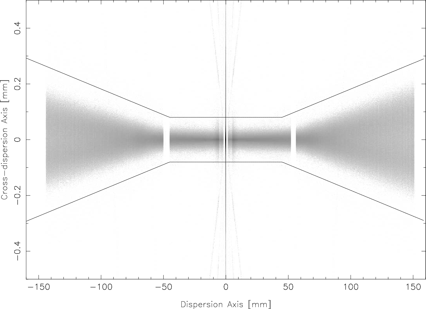 The LETG/HRC-S spectral extraction region has a 'bow tie' shape,
narrow in the middle and widening on the outer plates to accommodate the
inherent astigmatism of the LETG's Rowland-circle geometry.
The figure at right (vertical axis highly stretched)
is based on MARX simulations;
the true spatial distribution of the dispersed spectrum
differs in several small but sometimes significant ways from the ideal:
The LETG/HRC-S spectral extraction region has a 'bow tie' shape,
narrow in the middle and widening on the outer plates to accommodate the
inherent astigmatism of the LETG's Rowland-circle geometry.
The figure at right (vertical axis highly stretched)
is based on MARX simulations;
the true spatial distribution of the dispersed spectrum
differs in several small but sometimes significant ways from the ideal:
- The cross-dispersion profile (along the tg_d axis) is asymmetric.
- The spectrum has a slight time-dependent tilt (up to 4-pixel
errors at the longest wavelengths).
- The spectrum has a slight (<0.5 pixel) time-dependent curvature.
- Pipeline determinations of zeroth order may have errors of
up to ~0.5 pixel.
- In addition to tilt, curvature, and slight offsets,
the dispersed spectrum has a time-independent pattern
of tg_d offsets (~2.5 pixels peak-to-peak "wiggles")
as a function of position on the detector.
- Even when the position of 0th order is well determined
and tilt and wiggle have been removed,
the dispersed spectrum, particularly
on the outer plates, may be slightly (~0.5 pixel) offset in tg_d.
*** Check if there's a thermal
correlation. HZ43 residuals seem to correlate with month.
Together, these effects can add up to deviations
of more than ± 6 pixels
in the tg_d direction (near the plate ends), although errors
are more typically 1 or 2 pixels.
For comparison, the current extraction region half width is
12.45 pixels (80 μm, 5.31e-4 deg) in the central region.
At 170 Å the
half width is 42.1 pixels (270.7 μm, 19.96e-4 deg).
Motivation and Method
The intention of our analysis is to straighten and align dispersed spectra,
and then calibrate the intrinsic cross-dispersion profile. We can then
define a narrower spectral extraction region which will contain nearly the
same enclosed energy fraction (EEFRAC) as the current region
but a proportionally smaller
background signal. The result is a better calibrated EEFRAC
only 1-2% smaller than the original with ~25% (TBD) less background.
We use bright, frequently observed continuum sources
to provide complete wavelength coverage
with high signal. Mkn421 and PKS2155 are used for short wavelengths
(<~60 Å) and HZ43 for longer wavelengths. Emission lines from
Capella, a bright coronal source, are used to tie together the short-
and long-wavelength calibration. All the observations we use were
made on-axis (Yoffset=0) and were processed to Level 2 using the latest
CALDB. The
LETGS Background Filter
was then applied, and time periods with DTF<0.98 (indicating significant
background flaring) were removed to improve S/N. HRC background is also
spatially nonuniform during flares. (Show figure? BG crowned as f(crsu),
LESF shadow, nonuni as f(crsv?). Why would it be crowned across short
axis?)
tg_d profiles are extracted for each dispersion-axis tap (crsv)
with the implicit assumption that profiles are (over short spatial scales)
predominantly a function
of location along the detector rather than a function of wavelength.
Analysis of a few off-axis observations confirms this. Binning by
tap typically provides a few thousand events (and thus centroiding
errors of a couple/few percent of the profile FWHM) and good sampling
of the dispersed spectrum's wiggles. Within a tap, tg_d is binned
by 0.00005 degrees (~1.2 pixels) on the central plate and 0.00007
to 0.00010 degrees on the outer plates (where the profiles are
wider--see Fig. 1). Wider bins may obscure detail while narrower
bins may have too few counts, causing interpolation errors.
The findcenter.f program reads the tg_d profile data
and computes medians (50% of events below and above) as well
as tg_d values for cumulative fractions of
1, 2, 3, 4, 5, 10, and 25% (and 75 ... 99%)
of net (background-subtracted) events, with interpolation
between bins for greater accuracy. The background level
is determined from counts in the range
tg_d=-0.023:-0.013,0.012:0.0205 for the negative order and
tg_d=-0.026:-0.015,0.012:0.0205 for the positive order.
Background is not perfectly flat, but these ranges
provide a good estimate of the level under the
primary dispersed spectrum.
Cross-dispersion orders 1--4, important at short wavelengths
(see the faint "whiskers" of orders 1 and 2 in Fig. 1),
are excluded when determining the background level, but not
when determining the cumulative count fractions (which are relative to the
total counts falling interior to the background regions, i.e.,
tg_d=-0.013:0.012 for the negative order and
tg_d=-0.015:0.012 for the positive order).
Note that the cumulative count fractions calculated by
findcenter.f are not the same as CALDB EEFRACs.
The latter fractions are relative to the total diffracted
flux of the primary 1st order integrated over 2π steradians.
If there are no cross-dispersion orders in the X-ray region then
the EEFRACs will be ~0.905 times the findcenter.f EE fractions,
where 90.5% is the total power of the primary 1st order, which includes
diffraction from the coarse support structure but not cross-dispersion
orders from the fine-support structure.
For reference, the cross-dispersion orders contain ~9.5% of the
total flux, with 1.7% in 1st order, 1.6% in 2nd, 1.3% in 3rd,
1.0% in 4th, etc.
As another example,
if the 1st cross-dispersion orders are in the tg_d analysis range
and the findcenter.f cumulative count fraction is 0.95 then
the EEFRACS is (0.905+0.017)*0.95 = 0.876.
This is only approximate. A non-negligible fraction of
events (especially at high energies) are scattered beyond the
tg_d inspection region used by findcenter.f. I'll have to rely
on MARX/SAOSAC sims to estimate that.
0th Order positions
The CIAO tool celldetect is used in Standard Data Processing
to determine the position of 0th order, which is then used as the origin for
the grating coordinates tg_d and tg_r. Errors of a few tenths of a
pixel in 0th order are common in Archive data (although data processed
after Oct 2013--TBD***--use different celldetect parameter values that yield
better results). The easiest way to improve those positions is to
use dmstat on the 0th order position listed in the evt2
region block, e.g.,
dmlist "archive_evt2.fits[region]" data |grep circle
   Use the circle coordinates in the next step.
dmstat "/archive_evt2.fits[(x,y)=circle(xxx,yyy,12)][cols sky]"|grep mean
The improved 0th order position is then used to reprocess the data
by following
this or some other *** thread.
Tilts
After reprocessing the data using new 0th order positions we
extracted tg_d profiles for each crsv and then ran findcenter.f
to compute tg_d medians. To remove the wiggle from our results and
enable a better determination of the (relative) tilt of each spectrum
we computed the average tg_d median as f(crsv) for each source
and subtracted that curve from the results for each ObsID.
Results, grouped by source, are shown below.
|
|
|
|
|
Fig 2. tg_d medians vs crsv, after subtracting the average
tg_d median for each source. Tilts are therefore relative to the
average tilt for each source. For continuum sources, only points
with errors of less than 1e-5 degrees (about 1/4 pixel) are plotted.
Errors for Capella's lines' medians are explicitly shown.
|
As can be clearly seen in the left-panel plots,
LETG/HRC-S spectra have a time dependent tilt.
(LETG/ACIS spectra probably do too, but the extraction region is wider
and the spectra shorter so the effects are negligible.)
Right-panel plots show results after tilts (derived from
linear error-weighted fits) are removed.
Note that even after correcting the 0th order positions and tilts,
some spectra (e.g., 3rd right panel for HZ43) have a general tg_d
offset. This seems to be correlated with the time of year and may
therefore be a thermal effect. There also appears to be
a slight time-dependent curvature, particularly on the inner plate
(e.g., upward curvature for early Mkn421 observations and downward
for later).
The earliest observations also show relatively large
deviations in tg_d offsets and/or curvature near 0th order, but this
wavelength range is usually unimportant for LETG observations.
[See /data/letg4/bradw/EEFRACS2013/Mkn421/averesids.sm--exclude
0th, average resids, and plot vs time.]
Within each source-group, tilts are well determined relative to
the group average and we removed the tilt in each observation by
running a script called *** to adjust the tg_d value for every
event in a given observation's event file. All the files for
a given source were then combined using dmmerge
in order to improve statistics.
(The two weakest PKS2155 spectra were not included in that source's
combined file.)
Defining an absolute tilt is somewhat arbitrary because
of the spectral wiggles.
Because of minimal wavelength overlap of the continuum sources,
there is also some ambiguity in how tilts are measured on the
inner versus outer plates. Capella spectra, which have prominent
lines on all three plates, were analyzed to address the latter issue
but limited statistics (see error bars in Fig 2) prevented a
definitive calibration. We therefore adjusted the tilts of
the four composite spectra by eye in order to obtain the best
agreement among them (in both Figs. 3 and 4) while also aiming to make
the wiggles symmetric about tg_d=0 (Fig. 3).
In the overlap region
at wavelengths beyond |λ|~70|Å, higher order
diffraction contributes most of the events seen in the hard
continuum source spectra, which broadens the tg_d profile and
skews the median. We therefore ignore those results and use only
data from HZ43. Similar effects might
be expected just short of the C-K absorption edge (because 1st order
is much reduced) but we do not observe anything obvious. Likewise,
results from HZ43 become increasingly suspect toward shorter wavelengths
because of decreasing flux.
|
|
| Fig. 3. Median tg_d values for combined spectra, with tilt
and offset adjustments to make the wiggle symmetric about tg_d=0.
tg_d values are multipled by 1000 for convenience
and units are degrees. Tilts are in units of degrees per tap, also
multipled by 1000.
Legend example: blue points are for 18 combined HZ43 spectra,
with a tilt correction of 0.00090 and global offset of 0.043.
The composite wiggle curve is shown in black;
some points near 0th order and the ends of the inner plate were
adjusted by hand because the true errors are larger than indicated
by the purely statistical error bars. (The lower panel in the
linked figure plots the same data without the global offsets,
and therefore shows the true wiggle correction curve.)
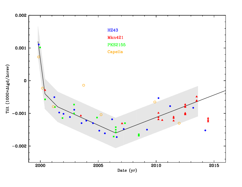
| Fig. 4. Time dependent tilts. Uncertainties on each point
(other than for Capella) are small,
so the observed scatter is real and probably caused
by observation-specific thermal conditions.
There is no apparent correlation with
aimpoint jumps.
The solid black line can be used to estimate the tilt in any observation,
and the gray band denotes the degree of uncertainty that would cause
a 1-pixel error at 170 Å.
|
With a consistent measure of tilt across all three plates, the
tilt-versus-time curves from all 4 sources can be plotted together,
as shown in Fig 4. The gray band represents a tilt uncertainty that
would cause 1 pixel of error at 170 Å (proportionally less
at shorter wavelengths), which is much larger than
any errors in the wiggle calibration. Error bars on the points in Fig. 4
are quite small, so the jump between the blue HZ43 points around
2010 is real. The cause of this jump and other scatter is unknown,
but probably thermal;
there is no correlation with aimpoint jumps or any other parameters
that we investigated. The 2007--2013 trend does not seem to continue in 2014.
Result: Consistent Spectra Suitable for Optimized Extraction Region
With the wiggle and time-dependent tilt thus calibrated an
observer can apply adjustments to any LETG/HRC-S observation
and obtain a corrected event file... *** blah blah.
- Determine an accurate 0th order position.
- Reprocess to level 2 (?)
- Apply the wiggle correction. The spectrum is now straight but
may be tilted.
- Determine the tilt correction from Fig. 4 and
run the *** script.
- Reextract spectrum using the optimized extraction region described
below.
- Note that only tg_d values are modified. Spectra will still have
tilts and wiggles in other coordinate systems, such as sky.
These corrections are only calibrated for on-axis obs's,
but they're probably OK for any conceivable off-axis pointing
because the PSF degradations will likely be larger than any
errors arising from using the on-axis calibration.
Errors on tg_d in the corrected L2 event file should be no more than
about 0.5 pixels on the central plate and 1.5 near the ends of the
outer plates. If the source is bright enough
one can probably reduce these errors to only a few
tenths of a pixel by measuring the residual tilt and overall tg_d offset
and applying another round of corrections.
A slightly narrower spectral extraction region could then be used
but the net benefit would be only a few percent reduction
in the included background.
For clarity, what's above here should only
talk about tg_d medians and fixing the event data (get better 0th order
position, remove wiggles and tilt). What comes next is recalibrating the
EEFRACs table and choosing an optimal extraction region. Add
data from KT Eri (20-40+ Å) and RS Oph (15-30 Å),
which have super-high rates (low BG, high stats) and no higher-order
contamination (unlike Mkn421). Make high-stat tg_d profiles,
carefully treat BG and Xdisp orders, extract new EEFRACs with
proper 2π normalization (and adjust HRC-S to get same EA),
specify optimized extraction region.
DTF filtering NOT applied to RS Oph or KT Eri data because
of telem saturation; in this case, BG is negligible even with
flaring and
DTF filtering reduces the S/N.
LSF distortion is not a concern for anything but 0th order.
New Extraction Region and EEFRAC Calibration
After applying tilt and wiggle corrections to the combined data we can
calibrate the tg_d profile, or cross-dispersion Line Spread Function,
and create new EEFRAC tables for the LSFPARMs files in the CALDB (give link),
along with a narrower spectral extraction region.
The hard-source spectra we used to calibrate spectral
tilt and wiggles have relatively strong higher orders, which will tend
to broaden the measured LSF. We therefore include observations of
the very bright continuum sources RS Oph (ObsIDs 7296, 7297) and
KT Eri (ObsIDs 12097, 12100, 12101, 12203) in our analysis.
RS Oph covers from 15-30 Å and KT Eri from 20 to ~50 Å
(see Fig. 8) and have essentially no higher order
contamination in those wavelength ranges. The observations we use
were obtained when those sources were extremely bright, often exceeding
the HRC-S telemetry limit. High rates can cause deformations in the
core of the 0th order PSF but did not affect the LSF of dispersed
spectra, except for ObsID 12203 (see Fig. 9) which we do not include in
further analysis. DTF filtering, which applied to Mkn421, PKS2155, and HZ43
data in order to eliminate periods of background flaring, was not
applied to RS Oph or KT Eri data because that would remove data during
the many periods of telemetry saturation. Note that background is almost
negligible during those very-high-rate observations.
|
|
|
| Fig. 8. Spectra used for central plate. The combined Mkn421
spectrum has by far the most counts but had the lowest (average)
counting rate, and therefore relatively more background.
It also has the largest contribution of higher order diffraction,
which makes the LSF slightly broader than it is for the ideal
1st order spectrum. The KT Eri observation 12203 had the highest
rate and its LSF was noticeably broader than the others (see
Fig. 9). |
Fig. 9. Comparison of background-subtracted LSFs (tg_d profiles)
around +25 Å.
Residual errors of up to 1/4 pixel in tg_d centroid were corrected
for these plots to enable easier comparisons
(but not in the evt files because such errors
are representative of what users can expect).
The LSF of Obsid 12203 is broader than the others and is not used
in our calibration. More detailed study at other wavelengths
confirms that data from other ObsIDs do not suffer from high-rate
distortions,
although the Mkn421 LSFs are broadened at some wavelengths
by higher order contributions.
(Key plot is upper left; others are sanity checks
that will just be confusing to other people so I should
remove them.) |
Fig. 10. Cross-dispersion orders;
profiles from - and + orders (primary and Xdisp) are combined.
Large X's mark peaks that were superseded by other data.
+ signs mark the
center of "background" regions on either side of a peak; note
that this background includes intrinsic HRC background and
underlying counts from the wings of the primary order.
Dotted line marks the detector background level.
The Mkn421 background levels were adjusted (- signs) as
described in the text. |
Cross-Dispersion Orders
As seen in Fig. 8, the short-wavelength range is only covered by
Mkn421, which has significant higher order contamination that affects
the LSF. An example, comparing to the "clean" LSF of KT Eri, may
be seen here (25-40 Å,
KT Eri in orange, Mkn421 in black). We can create model LSFs
and EEFRACs via interpolation in the problematic ranges, but this
requires calibration of the cross-dispersion orders diffracted
by the LETG fine-support structure. Cross-dispersion intensities
are also needed for proper normalization of the EEFRAC to 2π
diffracted flux.
[Why not use LETG/ACIS? Subarrays limit coverage of Xdisp orders
to ~1/2 of HRC-S and pileup often messes up normalization to 0th.
Also, I looked out to mX=12 with summed Mkn421 LETG/HRC (see
$EE/XdispCal2/plotgrass12.ps). Tough to set the BG but it looks
like 11 and 12 are significantly weaker than 10th.]
We used data from KT Eri and RS Oph as described above, along with
Mkn421 data between 5.5 and 8.4 Å. Rates shortward of 5.5 Å
drop rapidly so that 2nd order contamination in our chosen range
is very small, and 3rd order is even less. The large number of
events in this data set (about 550,000 in 0th order) provides
adequate statistics to see to mX=10, with hints of 11th order
(Fig. 10).
Event-file data were divided into thin triangular wedges
(source center at pointy end) so that events of any given Xdisp
order would all be collected together regardless of wavelength.
Wavelength ranges for each source were chosen to provide optimal
combinations of order coverage and S/N. Data from + and - primary
orders and + and - Xdisp orders were combined, with the tg_d limit
of ±0.021 deg chosen to maintain a flat detector background
(i.e., without dither losses near the edges). Data were also
analyzed separately (+ vs -) to confirm that results were
the same within errors.
Skipping over much detail that I'll write up on some other page
some day...The Mkn421 short-wavelength orders are so close together
that their wings overlap and the real background levels can not be
seen. We therefore adjusted them so that results for orders 3 and 4
matched those from RS Oph and KT Eri, scaling the background adjustments
for each peak by its intensity. The net change was to increase each
peak by about 5%. 0th order intensity was determined by subtracting
all higher Xdisp peaks from the full-width total counts, blah blah.
The SRON final calibration report
suggests (pg 81, Fig 7.1) that Xdisp orders reach a minimum around
mX=11 with damped oscillation beyond that. Based on fits to our
results using a sum of squared sinc functions and the SRON report's
caveats about PSF wings and background we believe that their results
(using Al-K) are too high for orders 1, 2, and >10. Our model predicts that
orders beyond 10 have a combined intensity of 0.0049 relative to 0th.
Results are listed below. (Plots and analysis in
/data/letg4/bradw/EEFRACS2013/XdispCal2.)
Order	Intensity relative to 0th, with statistical uncertainty
1       0.00837  0.00010  (but 0.00759 ± 0.00035 for HZ43 70-82 Å)
	0.00831  0.00010   if HZ43 results included--I use this
2       0.00781  0.00010
3       0.00678  0.00010
4       0.00569  0.00016
5       0.00405  0.00013
6       0.00316  0.00013
7       0.00191  0.00012
8       0.00113  0.00012
9       0.00086  0.00012
10      0.00046  0.00011
>10     0.0049	 ?
Total   0.04506 ±0.00041  * 2 for both sides --> 0.0901 +/- 0.0008
	not including uncertainty in orders beyond mX=10.
We find that Xdisp orders have a total of 9% as much flux as the
primary order, vs. the expected 11%. The 1st order intensity may also
differ depending on wavelength, even at low energies where
grating-bar transparency should not be an issue: 0.84% of 0th
for wavelengths 15-39 Å and 0.76% for 70-82 Å,
a 2.1σ difference. It is not clear if this
result is significant or not. The SRON report noted
differences between Al-K and O-K results but their
significance was also questionable.
Possible nonnegligible systematic error sources:
nonlinear nonuniformity in QE in the Xdisp direction;
nonlinear nonuniform detector background in the Xdisp direction;
primary higher order contamination in the Mkn421 5.5-8.4 Å spectrum.
Implications: I think that any errors in Xdisp (and raytrace)
modeling would affect our primary 1st order calibration in such
a way that errors in EEFRACs would cancel out and yield the same EA.
I should study the LSF and Xdisp orders in LETG/ACIS data at some point.
Hmmm, this DOES affect the LETG/ACIS EA because it's absolutely
calibrated. I'll have to check but I think my EEFRAC work
assumed 90.5% in the main order--half a percent error is
nothing, and the uncertainty in my Xdisp calib is probably
similar.
Last update 5/12/14. Plots below will be updated with improved results.
Data from all 5 continuum sources were binned in few-Å slices
to obtain roughly TBD** counts per bin and their tg_d profiles extracted
as before. The program contours.f was used to
measure cumulative count fractions and blah blah... see Figure 6 (for
now, but I need to make a new one).
Medians are also
shown for uncorrected Archive data from two observations with extreme tilts
(ObsIDs 59 and 8274, corresponding to the highest and lowest points
in Fig. 4).
|
|
| Fig. 6. Cumulative count fractions of
corrected data from combined Mkn421 and combined HZ43 observations.
The cross-dispersion 1st order is shown in light gray (also
seen with 2nd order as the faint "whiskers" in Fig. 1).
Solid black line is the current spectral extraction region.
|
Fig 7. tgd profiles for HZ43 ObsID59 before correcting tilt.
Remake this using composite HZ43 and Mkn421 files,
and swap +/- to left/right.
|
Meeting notes (7/29/13)
- Mike et al have some ideas about what's causing the wiggles and tilt
but nothing very firm. Net effect on astrometry for this and
other instrument configs seems pretty unimportant and/or not
worth the large effort to try to calibrate it, if even possible.
- Dave will compare three methods of determining 0th order position:
celldetect (current SDP method), dmstat on a 12-pix-radius
circle centered on the SDP position, and an adaptation of
tg_findzo, which uses the transfer streak in xETG/ACIS data.
Pete has repro'd data using the dmstat method and
I will redo my analysis with those and let Dave know how
things look, a la Fig 3.
- The time-dep tilt can be handled in CIAO by changing an angle in the
geom file. Pete uses a perl script. We can probably use a simple
time-dep curve to adequately assign a tilt for any observation, but
might want to come up with a method for determining a more precise
tilt for each obs. The latter is what Pete does now but we
would need a simpler method for general users.
- The wiggles, aka "fixed pattern," should be treated right after the
degapping using a f(crsv) correction with a lookup table,
adjusting chipx across the full width of the detector.
For my analysis, Pete can write a perl script to adjust
chipx (or tgd to avoid going so so far back in the repro.)
(For public use it will be easier to determine an
exact tilt if the wiggles are fixed first.)
- The current EEFRACS tables don't require profile
symmetry about tgd=0, but do assume a symmetric extraction
region. EE contours are not symmetric. This doesn't
matter much with the current relatively wide extraction region
but an optimal, narrower extraction region will not be symmetric.
There was no consensus on how to handle this;
one option is to use the wide-region
EEFRACS and then apply a correction. One could also specify
the wiggle corrections to make things symmetric for a specific
extraction region, or use a symmetric region with asymmetric
EE contours but have the EEFRACS table give the net EE as if
the contours were symmetric.
- The net result of all these corrections will be to enable a
~25% narrower extraction region, reducing BG by the same
amount with a TBD tiny change (probably a reduction of <1%)
in X-ray extraction efficiency. (I will also design an even
narrower region to use for gain analysis, in which minimizing
the BG is very important but EEFRACS calibration isn't.)
Given the modest benefit
and limited SDS manpower, this project will not be a high
priority for implementation in CIAO/CALDB. I plan to provide
these improvements as contributed software/thread. This
page will be revised to serve as user documentation.